Multivariate normal: the precision matrix
Matthew Stephens
University of ChicagoJanuary 12, 2026
Last updated: 2026-02-11
Checks: 7 0
Knit directory: fiveMinuteStats/analysis/
This reproducible R Markdown analysis was created with workflowr (version 1.7.1). The Checks tab describes the reproducibility checks that were applied when the results were created. The Past versions tab lists the development history.
Great! Since the R Markdown file has been committed to the Git repository, you know the exact version of the code that produced these results.
Great job! The global environment was empty. Objects defined in the global environment can affect the analysis in your R Markdown file in unknown ways. For reproduciblity it’s best to always run the code in an empty environment.
The command set.seed(12345) was run prior to running the
code in the R Markdown file. Setting a seed ensures that any results
that rely on randomness, e.g. subsampling or permutations, are
reproducible.
Great job! Recording the operating system, R version, and package versions is critical for reproducibility.
Nice! There were no cached chunks for this analysis, so you can be confident that you successfully produced the results during this run.
Great job! Using relative paths to the files within your workflowr project makes it easier to run your code on other machines.
Great! You are using Git for version control. Tracking code development and connecting the code version to the results is critical for reproducibility.
The results in this page were generated with repository version 4ec29db. See the Past versions tab to see a history of the changes made to the R Markdown and HTML files.
Note that you need to be careful to ensure that all relevant files for
the analysis have been committed to Git prior to generating the results
(you can use wflow_publish or
wflow_git_commit). workflowr only checks the R Markdown
file, but you know if there are other scripts or data files that it
depends on. Below is the status of the Git repository when the results
were generated:
Ignored files:
    Ignored:    analysis/bernoulli_poisson_process_cache/
Note that any generated files, e.g. HTML, png, CSS, etc., are not included in this status report because it is ok for generated content to have uncommitted changes.
These are the previous versions of the repository in which changes were
made to the R Markdown (analysis/normal_markov_chain.Rmd)
and HTML (docs/normal_markov_chain.html) files. If you’ve
configured a remote Git repository (see ?wflow_git_remote),
click on the hyperlinks in the table below to view the files as they
were in that past version.
| File | Version | Author | Date | Message |
|---|---|---|---|---|
| Rmd | 4ec29db | Peter Carbonetto | 2026-02-11 | Generated pdf version of normal_markov_chain vignette. |
| html | 5f62ee6 | Matthew Stephens | 2019-03-31 | Build site. |
| Rmd | 0cd28bd | Matthew Stephens | 2019-03-31 | workflowr::wflow_publish(all = TRUE) |
| html | 34bcc51 | John Blischak | 2017-03-06 | Build site. |
| Rmd | 5fbc8b5 | John Blischak | 2017-03-06 | Update workflowr project with wflow_update (version 0.4.0). |
| Rmd | 391ba3c | John Blischak | 2017-03-06 | Remove front and end matter of non-standard templates. |
| html | 8e61683 | Marcus Davy | 2017-03-03 | rendered html using wflow_build(all=TRUE) |
| html | 5d0fa13 | Marcus Davy | 2017-03-02 | wflow_build() rendered html files |
| Rmd | d674141 | Marcus Davy | 2017-02-26 | typos, refs |
| html | 0cd34f6 | stephens999 | 2017-02-21 | add figure and html |
| Rmd | b12c5ac | stephens999 | 2017-02-21 | Files commited by wflow_commit. |
| html | f196599 | stephens999 | 2017-02-19 | Build site. |
| Rmd | e778974 | stephens999 | 2017-02-19 | Files commited by wflow_commit. |
| html | c3b365a | John Blischak | 2017-01-02 | Build site. |
| Rmd | 67a8575 | John Blischak | 2017-01-02 | Use external chunk to set knitr chunk options. |
| Rmd | 5ec12c7 | John Blischak | 2017-01-02 | Use session-info chunk. |
| Rmd | 294d219 | stephens999 | 2016-02-16 | add normal markov chain example |
See here for a PDF version of this vignette.
Prerequisites
You should be familiar with the multivariate normal distribution and the idea of conditional independence, particularly as illustrated by a Markov chain.
Overview
This vignette introduces the precision matrix of a multivariate normal. It also illustrates its key property: the zeros of the precision matrix correspond to conditional independencies of the variables.
Definition, and statement of key property
Let \(X = (X_1, \ldots, X_n)\) be a multivariate normal random variable with covariance matrix \(\Sigma\).
The precision matrix, \(\Omega\), is simply defined to be the inverse of the covariance matrix: \[ \Omega := \Sigma^{-1}. \]
The key property of the precision matrix is that its zeros tell you about conditional independence. Specifically, \[ \Omega_{ij} = 0 \text{ if and only if } X_i \text{ and } X_j \text{ are conditionally independent given all other coordinates of } X. \]
It may help to compare this with the analogous property of the covariance matrix: \[ \Sigma_{ij}=0 \text{ if and only if } X_i \text{ and } X_j \text{ are independent}. \]
That is, whereas zeros of the covariance matrix tell you about independence, zeros of the precision matrix tell you about conditional independence.
Example: a normal Markov chain
Consider a Markov chain \(X_1, X_2, \dots\), where the transitions are given by \(X_{t+1} \mid X_{t} \sim N(X_{t},1)\). You might think of this Markov chain as a type of “random walk”: given the current state, the next state is obtained by adding a random normal value (with mean 0 and variance 1).
The following code simulates a realization of this Markov chain, starting from an initial state \(X_1 \sim N(0,1)\), and plots it.
set.seed(100)
sim_normal_mc <- function (T = 1000) {
  x <- rep(0,T)
  x[1] <- rnorm(1)
  for (t in 2:T)
    x[t] <- x[t-1] + rnorm(1)
  return(x)
}
plot(sim_normal_mc(1000),xlab = "time",ylab = "x")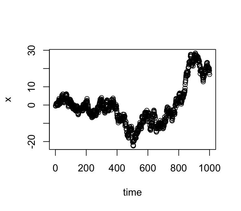
The normal Markov chain as a multivariate normal
If you think a little, you should be able to see that the above random walk simulation is actually simulating from a 1000-dimensional multivariate normal distribution!
Why? Well, let’s write each of the \(N(0,1)\) variables generated using
rnorm() in our code as \(Z_1,
Z_2, \dots\). Then we have \[
\begin{aligned}
X_1 &= Z_1 \\
X_2 &= X_1 + Z_2 = Z_1 + Z_2 \\
X_3 &= X_2 + Z_3 = Z_1 + Z_2 + Z_3,
\end{aligned}
\] and so on.
So we can write \(X = AZ\), where \(A\) is the following \(1000 \times 1000\) matrix: \[ A = \begin{pmatrix} 1 & 0 & 0 & 0 & \cdots \\ 1 & 1 & 0 & 0 & \cdots \\ 1 & 1 & 1 & 0 & \cdots \\ \vdots \end{pmatrix}. \]
Let’s take a look at what the covariance matrix \(\Sigma\) looks like. (We can get a good idea from looking at the top left corner of the matrix.)
A <- matrix(0,1000,1000)
for(i in 1:1000)
  A[i,] <- c(rep(1,i),rep(0,1000 - i))
Sigma <- A %*% t(A)
Sigma[1:10,1:10]
#       [,1] [,2] [,3] [,4] [,5] [,6] [,7] [,8] [,9] [,10]
#  [1,]    1    1    1    1    1    1    1    1    1     1
#  [2,]    1    2    2    2    2    2    2    2    2     2
#  [3,]    1    2    3    3    3    3    3    3    3     3
#  [4,]    1    2    3    4    4    4    4    4    4     4
#  [5,]    1    2    3    4    5    5    5    5    5     5
#  [6,]    1    2    3    4    5    6    6    6    6     6
#  [7,]    1    2    3    4    5    6    7    7    7     7
#  [8,]    1    2    3    4    5    6    7    8    8     8
#  [9,]    1    2    3    4    5    6    7    8    9     9
# [10,]    1    2    3    4    5    6    7    8    9    10
Now let us examine the precision matrix, \(\Omega\), which recall is the inverse of \(\Sigma\). Again we just show the top left corner of the precision matrix here.
Omega <- chol2inv(chol(Sigma))
Omega[1:10,1:10]
#       [,1] [,2] [,3] [,4] [,5] [,6] [,7] [,8] [,9] [,10]
#  [1,]    2   -1    0    0    0    0    0    0    0     0
#  [2,]   -1    2   -1    0    0    0    0    0    0     0
#  [3,]    0   -1    2   -1    0    0    0    0    0     0
#  [4,]    0    0   -1    2   -1    0    0    0    0     0
#  [5,]    0    0    0   -1    2   -1    0    0    0     0
#  [6,]    0    0    0    0   -1    2   -1    0    0     0
#  [7,]    0    0    0    0    0   -1    2   -1    0     0
#  [8,]    0    0    0    0    0    0   -1    2   -1     0
#  [9,]    0    0    0    0    0    0    0   -1    2    -1
# [10,]    0    0    0    0    0    0    0    0   -1     2
Notice all the zeros in the precision matrix. This is because of the conditional independencies that occur in a Markov chain. In a Markov chain (any Markov chain), the conditional distribution of \(X_t\) given the other \(X_s\) (\(s \neq t\)) depends only on its neighbors \(X_{t-1}\) and \(X_{t+1}\). That is, \(X_{t}\) is conditionally independent of all other \(X_s\) given \(X_{t-1}\) and \(X_{t+1}\). This is exactly what we are seeing in the precision matrix above: the non-zero elements of the \(t\)th row are at coordinates \(t-1,t\) and \(t+1\).
Addendum: interpretation of \(\Omega\) in terms of conditional mean of \(X_i\)
The following fact is also useful, both in practice and for intuition.
Suppose \(X \sim N_r(0,\Omega^{-1})\), where the subscript \(r\) indicates that \(X\) is \(r\)-variate.
Let \(Y_1\) denote the first coordinate of \(X\), and let \(Y_2\) denote the remaining coordinates, that is, \(Y_2:= (X_2, \dots, X_r)\). Further let \(\Omega_{12}\) denote the \(1 \times (r-1)\) submatrix of \(\Omega\) that consists of row 1 and columns 2 through \(r\).
The conditional distribution of \(Y_1 \mid Y_2\) is (univariate) normal with mean \[ E[Y_1 \mid Y_2] = -\Omega_{12} Y_2 / \Omega_{11} \] and variance \(1/\Omega_{11}\).
Of course, there is nothing special about \(X_1\): a similar result applies for any \(X_i\). You just have to replace \(\Omega_{11}\) with \(\Omega_{ii}\) and define \(\Omega_{12}\) to be the \(i\)th row of \(\Omega\) with all columns except column \(i\).
Application
An application of this is imputation of missing values: suppose one of the \(X\) values is missing, say \(X_i\) is missing, but you know the covariance matrix and all the other \(X\) values. Then you could impute \(X_i\) by its conditional mean, which is a simple linear combination of the other values that can be read directly off the \(i\)th row of the precision matrix. This idea is the essence of Kriging.
Example
Consider the Markov chain above. The conditional distribution of \(X_1\) given all other \(X\) values is given by \[ X_1 \mid X_2, X_3, \dots, X_{1000} \sim N(X_2/2, 1/2). \]
And the conditional distribution of \(X_2\) given all other \(X\) values is \[ X_2 \mid X_1, X_3, X_4, \ldots, X_{1000} \sim N((X_1+X_3)/2, 1/2). \] And similarly for \(X_i\), \(i = 3, \ldots, 1000\). The intuition is that, if we wanted to guess what the value of \(X_i\) were given all other \(X\)’s, the best guess would be the average of its neighbours.
sessionInfo()
# R version 4.3.3 (2024-02-29)
# Platform: aarch64-apple-darwin20 (64-bit)
# Running under: macOS 15.7.1
#
# Matrix products: default
# BLAS:   /Library/Frameworks/R.framework/Versions/4.3-arm64/Resources/lib/libRblas.0.dylib
# LAPACK: /Library/Frameworks/R.framework/Versions/4.3-arm64/Resources/lib/libRlapack.dylib;  LAPACK version 3.11.0
#
# locale:
# [1] en_US.UTF-8/en_US.UTF-8/en_US.UTF-8/C/en_US.UTF-8/en_US.UTF-8
#
# time zone: America/Chicago
# tzcode source: internal
#
# attached base packages:
# [1] stats     graphics  grDevices utils     datasets  methods   base
#
# loaded via a namespace (and not attached):
#  [1] vctrs_0.6.5       cli_3.6.5         knitr_1.50        rlang_1.1.6
#  [5] xfun_0.52         stringi_1.8.7     promises_1.3.3    jsonlite_2.0.0
#  [9] workflowr_1.7.1   glue_1.8.0        rprojroot_2.0.4   git2r_0.33.0
# [13] htmltools_0.5.8.1 httpuv_1.6.14     sass_0.4.10       rmarkdown_2.29
# [17] evaluate_1.0.4    jquerylib_0.1.4   tibble_3.3.0      fastmap_1.2.0
# [21] yaml_2.3.10       lifecycle_1.0.4   whisker_0.4.1     stringr_1.5.1
# [25] compiler_4.3.3    fs_1.6.6          Rcpp_1.1.0        pkgconfig_2.0.3
# [29] later_1.4.2       digest_0.6.37     R6_2.6.1          pillar_1.11.0
# [33] magrittr_2.0.3    bslib_0.9.0       tools_4.3.3       cachem_1.1.0