True Signal vs Correlated Null: Identifiability & Small Effects

Identifiablity of true signals from correlated noise

We’ve shown that in many real data sets when we have correlated null \(z\) scores, we can fit their empirical distribution with Gaussian and its derivatives.

But what if we have true signals instead of the global null? Theoretically, any distribution can be decomposed by Gaussian and its derivatives, also called Edgeworth series or Edgeworth expansion. We’ve shown that the Dirac delta function \(\delta_z\) and the associated \(0\)-\(1\) step function can be decomposed by Gaussian derivatives. Essentially all distributions can be represented by (usually infinitely many) \(\delta_z\), and thus be decomposed by Gaussian and its derivatives. There is a rich literature on this topic, probably of further use to this project.

Now the more urgent problem is: can true signals also be fitted by Gaussian derivatives in a similar way as correlated null? Let normalized weights \(W_k^s = W_k\sqrt{k!}\). As shown previously, under correlated null, the variance \(\text{var}(W_k^s) = \alpha_k = \bar{\rho_{ij}^k}\). Thus, under correlated null, the Gaussian derivative decomposition of the empirical distribution should have “reasonable” weights of similar decaying patterns.

If it turns out Gaussian derivatives with limited orders (say, \(K \leq 10\)) and reasonable normalized weights are only able to fit the empirical correlated null, but nothing else, then properly regularized Gaussian derivatives can be readily used to control the usually correlated noise, which are correlated null, and leave the signal to ash. But if true signals can also be fitted this way, the identifiability of true signals from correlated noise becomes an issue.

Let’s start with the simplest case: \(z \sim N(0, \sqrt{2}^2)\) independently. This data set can be seen as generated as follows.

\[ \begin{array}{c} \beta_j \sim N(0, 1)\\ z_j \sim N(\beta_j, 1) \end{array} \]

That is, a \(N(0, 1)\) true signal is polluted by a \(N(0, 1)\) noise.

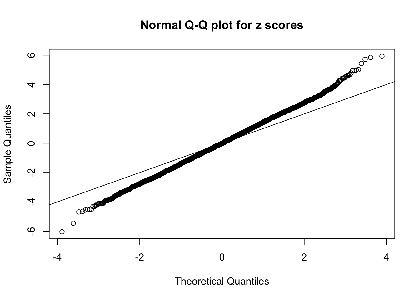
Illustration

n = 1e4
m = 5
set.seed(777)
zmat = matrix(rnorm(n * m, 0, sd = sqrt(2)), nrow = m, byrow = TRUE)

library(ashr)
source("../code/ecdfz.R")
res = list()
for (i in 1:m) {
  z = zmat[i, ]
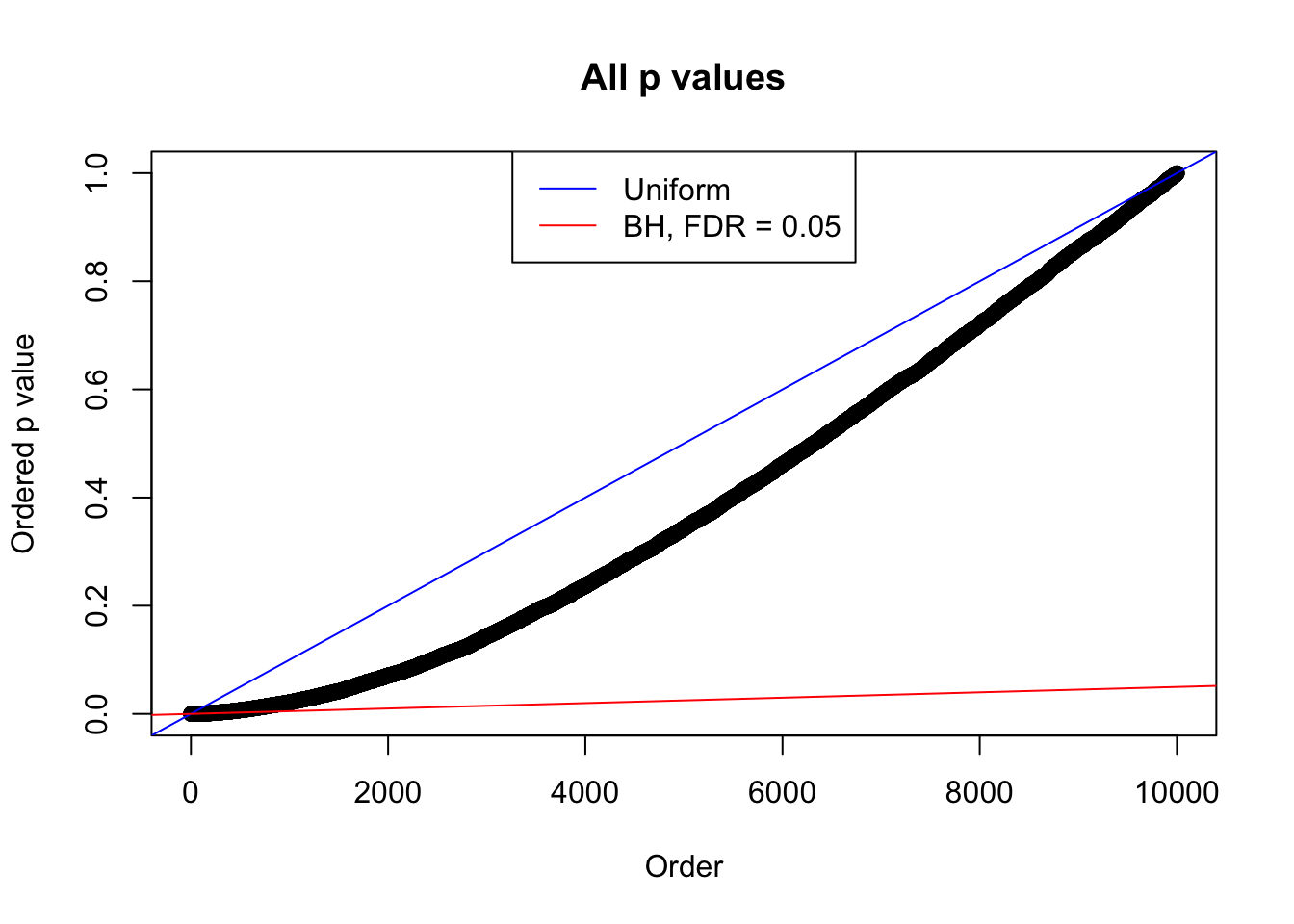
  p = (1 - pnorm(abs(z))) * 2
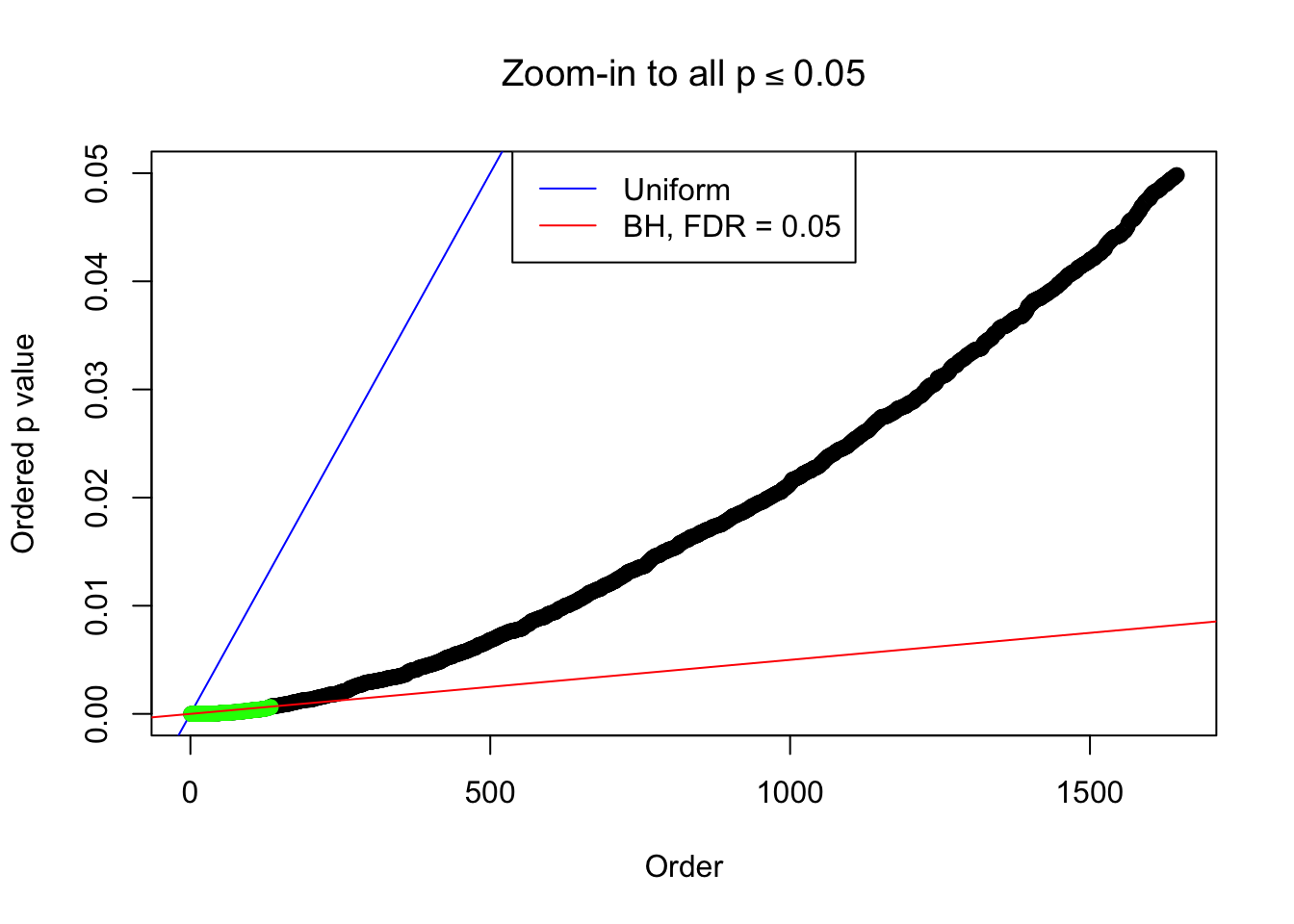
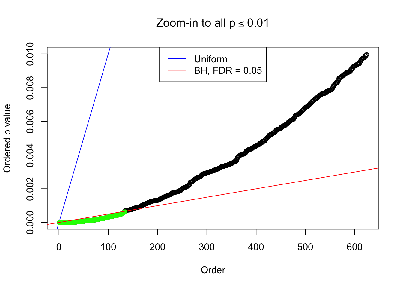
  bh.fd = sum(p.adjust(p, method = "BH") <= 0.05)
  pihat0.ash = get_pi0(ash(z, 1, method = "fdr"))
  ecdfz.fit = ecdfz.optimal(z)
  res[[i]] = list(z = z, p = p, bh.fd = bh.fd, pihat0.ash = pihat0.ash, ecdfz.fit = ecdfz.fit)
}

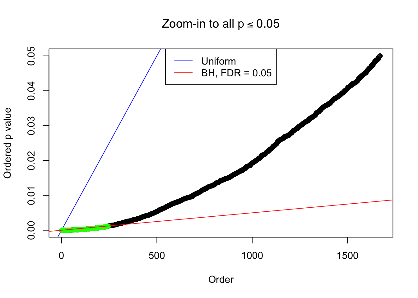
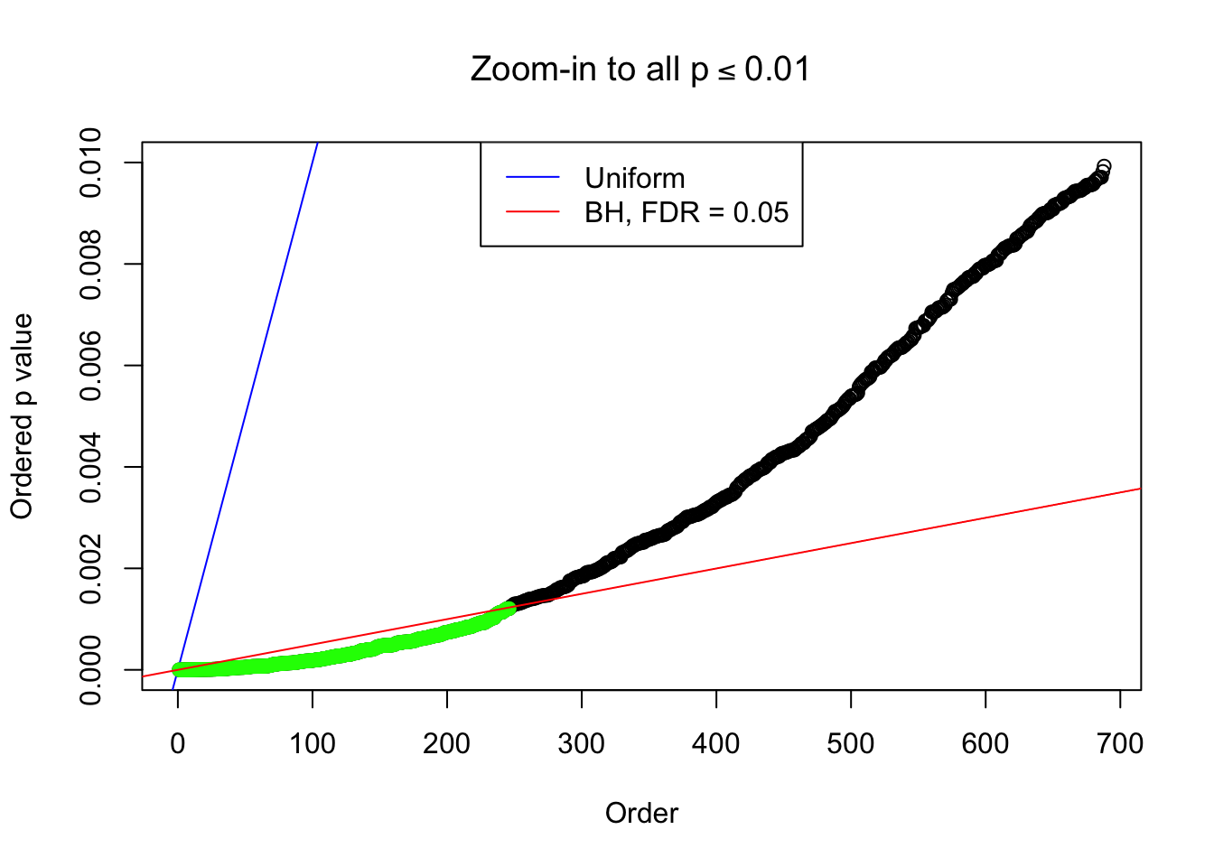
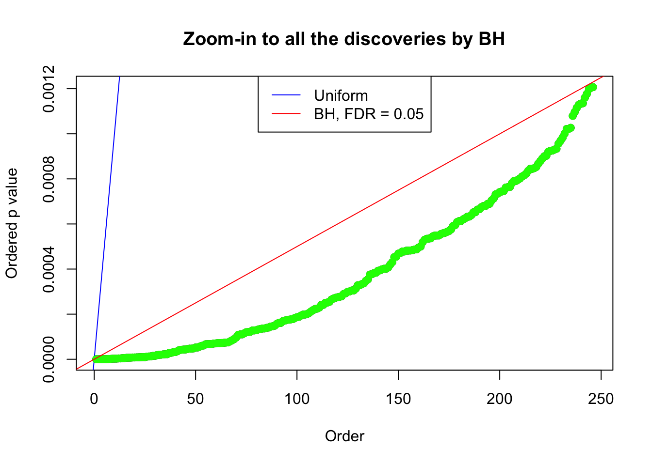
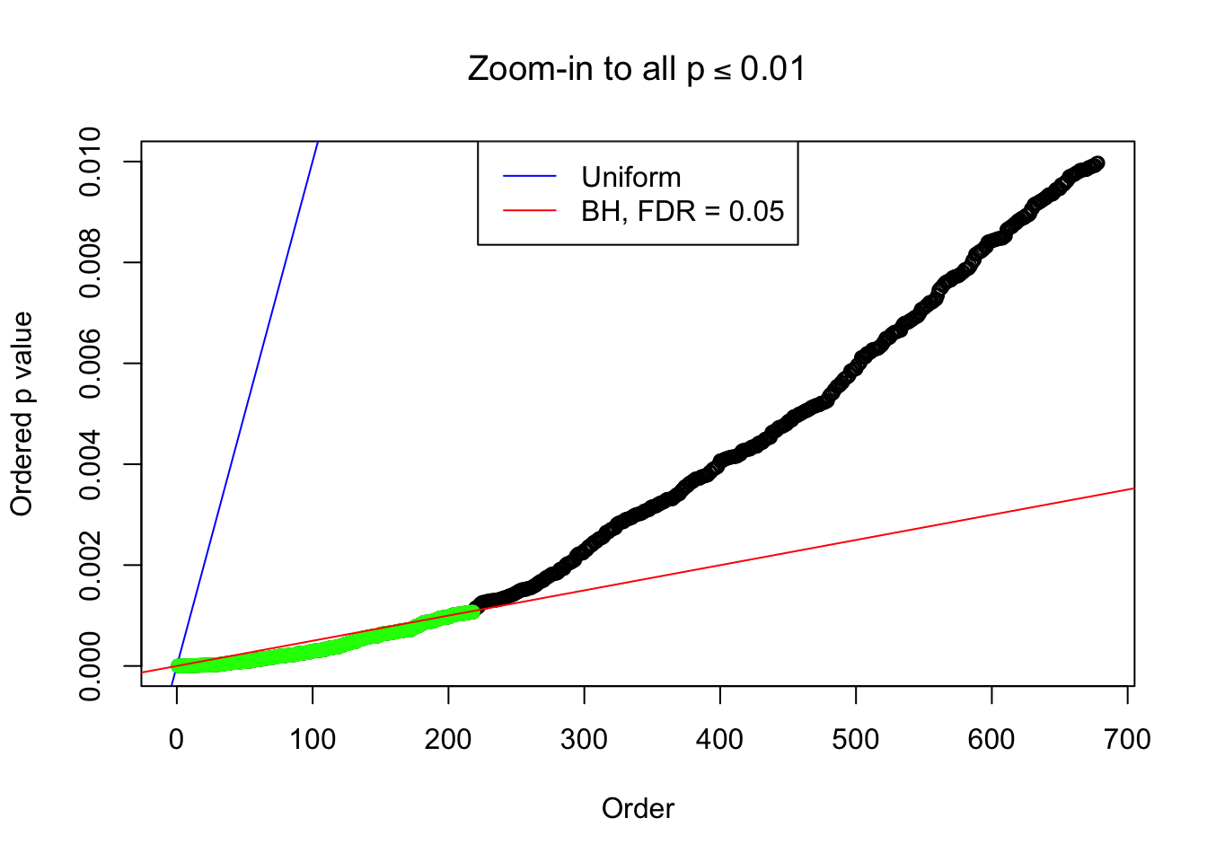
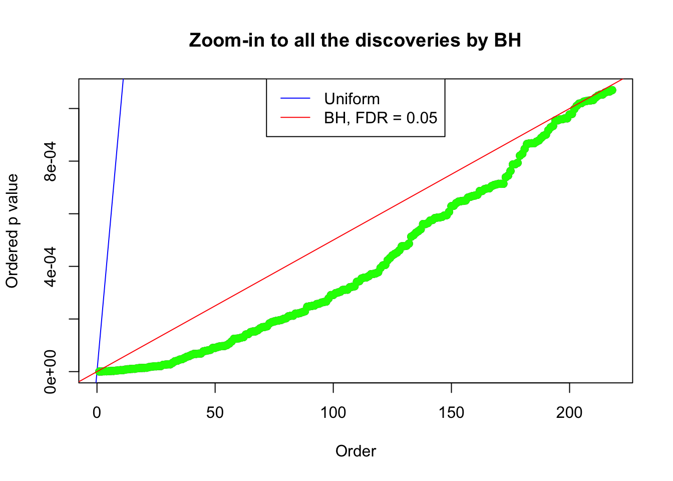
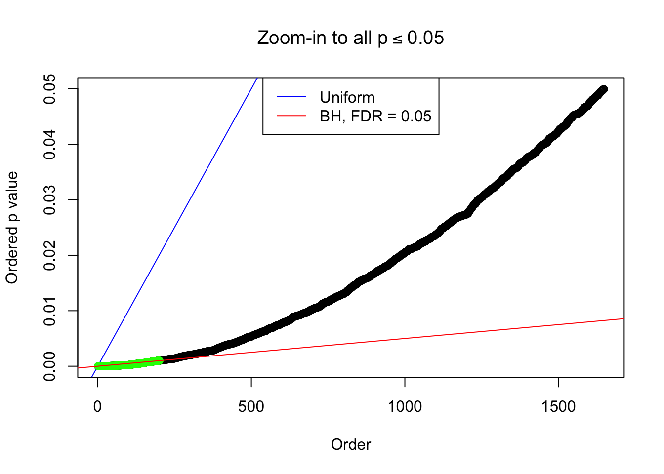
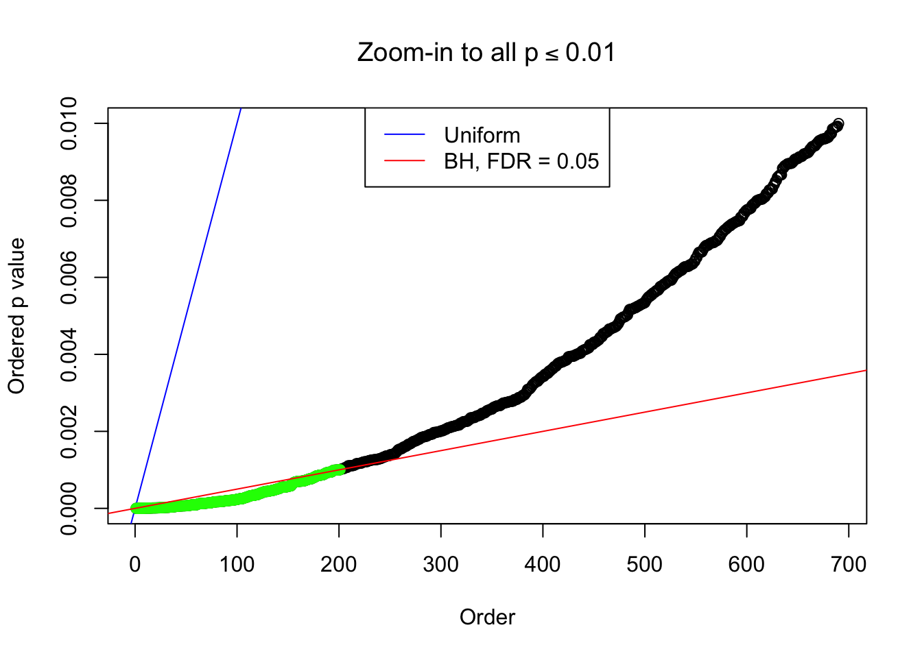
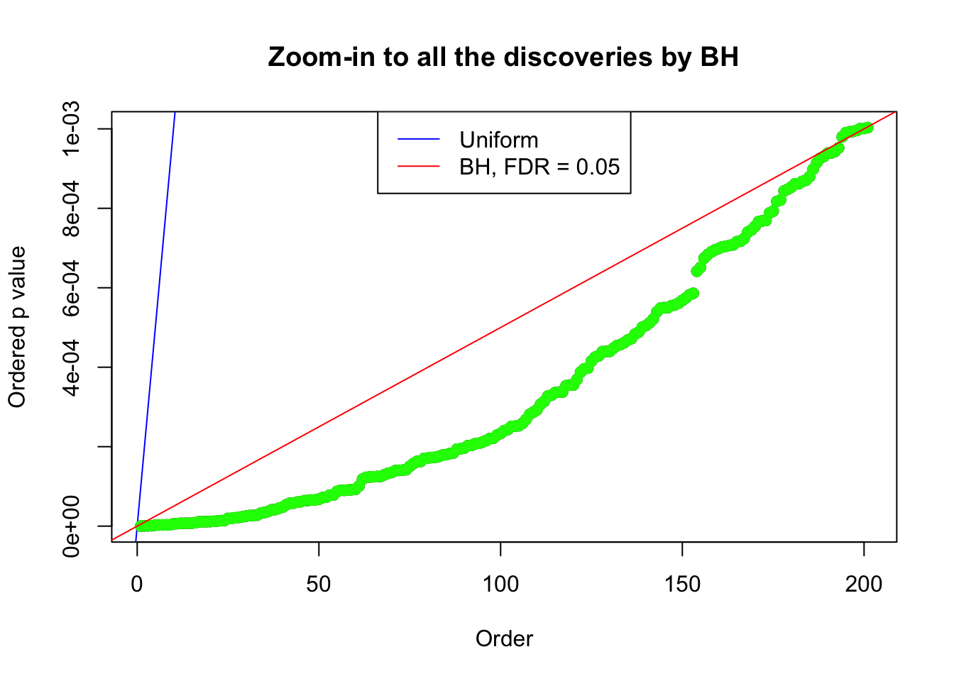
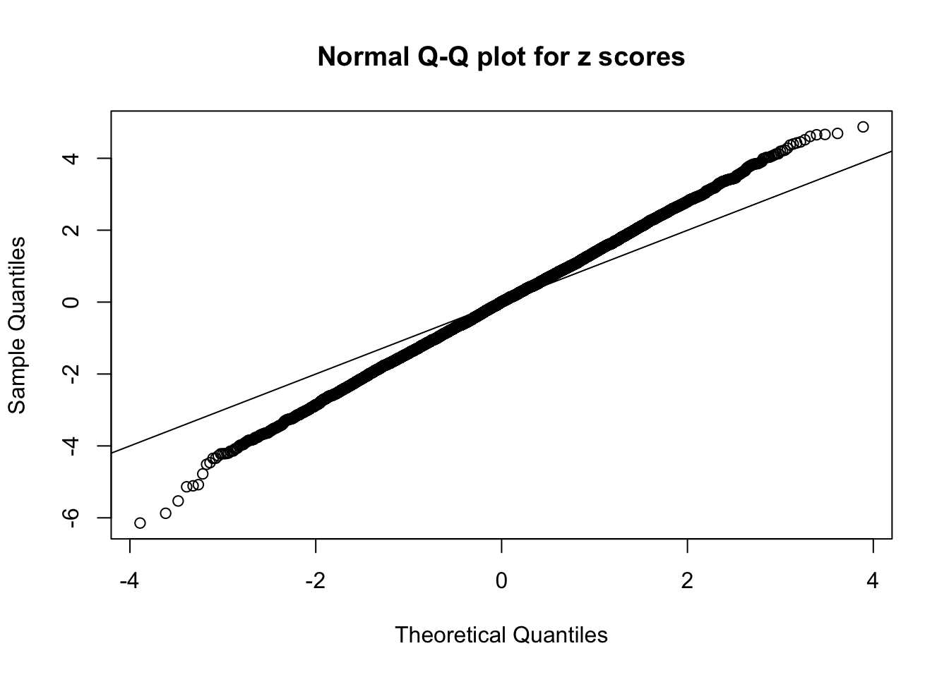
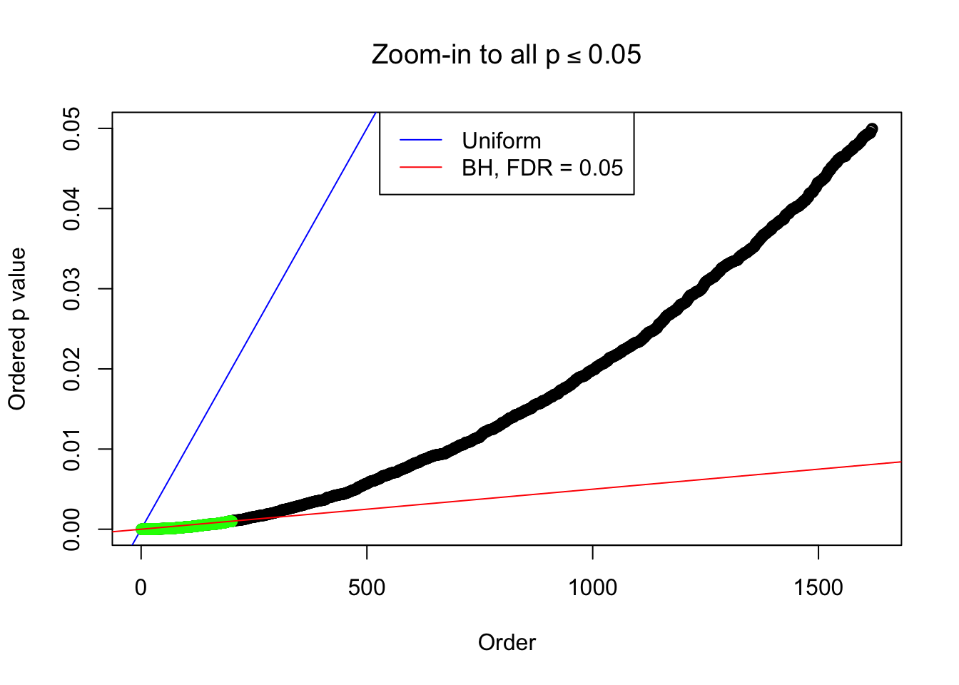
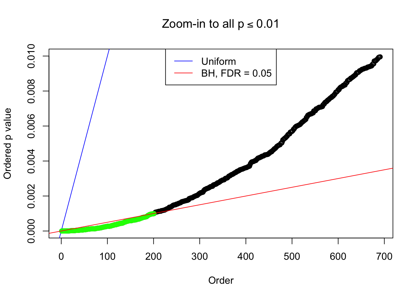
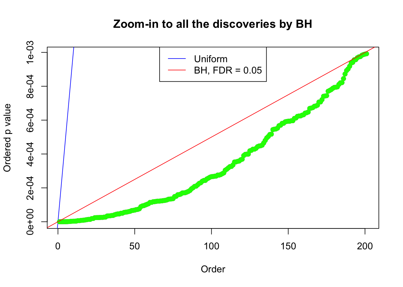
Example 1 : Number of Discoveries: 246 ; pihat0 = 0.3245191 
Log-likelihood with N(0, 2): -17704.62 
Log-likelihood with Gaussian Derivatives: -17702.15 
Log-likelihood ratio between true N(0, 2) and fitted Gaussian derivatives: -2.473037 
Normalized weights:
1 : -0.0126888368547959 ; 2 : 0.717062378249889 ; 3 : -0.0184536200134752 ; 4 : 0.649465525394262 ; 5 : 0.00859163522314002 ; 6 : 0.521325079359314 ; 7 : 0.0334885164431775 ; 8 : 0.22636494735755 ;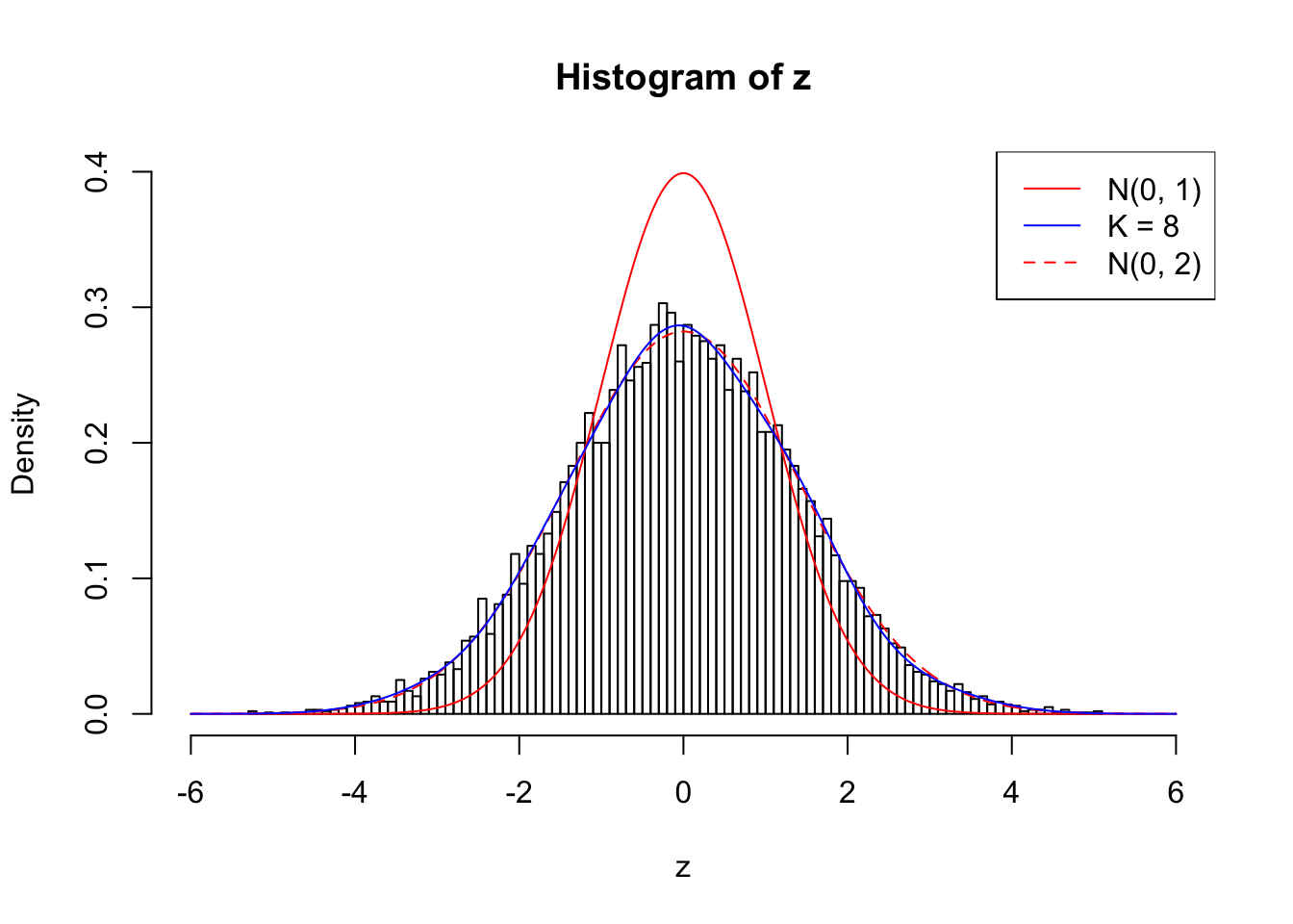

Zoom in to the left tail: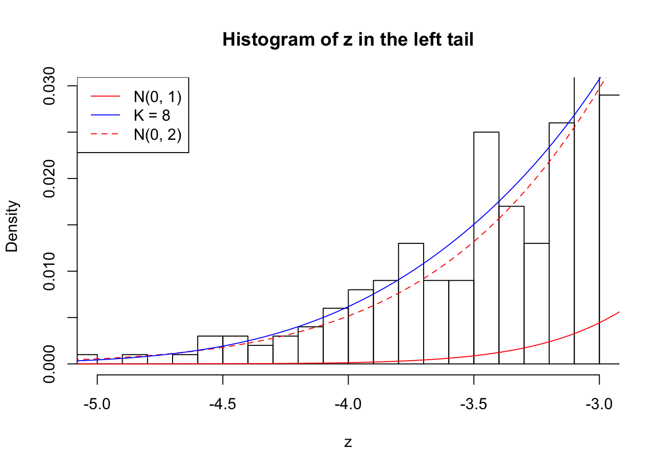

Zoom in to the right tail: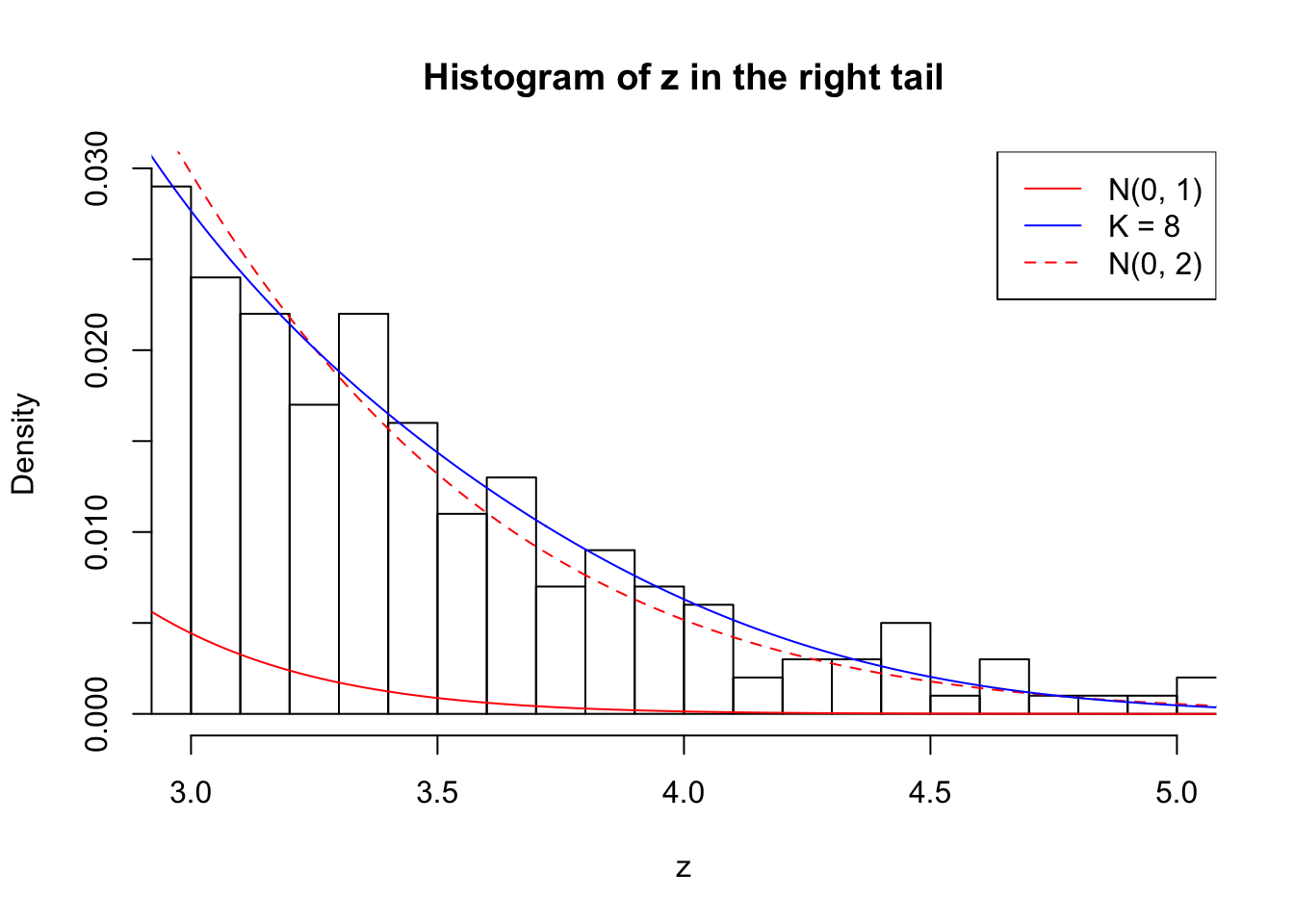

Example 2 : Number of Discoveries: 218 ; pihat0 = 0.3007316 
Log-likelihood with N(0, 2): -17620.91 
Log-likelihood with Gaussian Derivatives: -17618.13 
Log-likelihood ratio between true N(0, 2) and fitted Gaussian derivatives: -2.787631 
Normalized weights:
1 : 0.0102680011779709 ; 2 : 0.696012169853609 ; 3 : 0.0113000171720435 ; 4 : 0.544236663386519 ; 5 : -0.0208432030918437 ; 6 : 0.359654087688657 ; 7 : 0.00449356234470338 ; 8 : 0.129368209367989 ;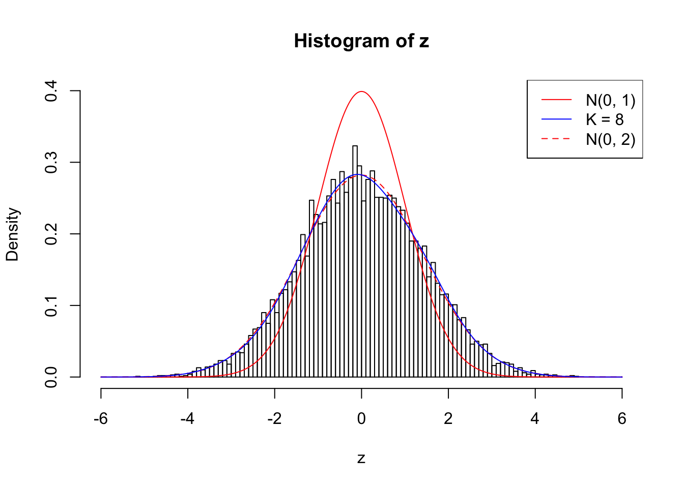

Zoom in to the left tail: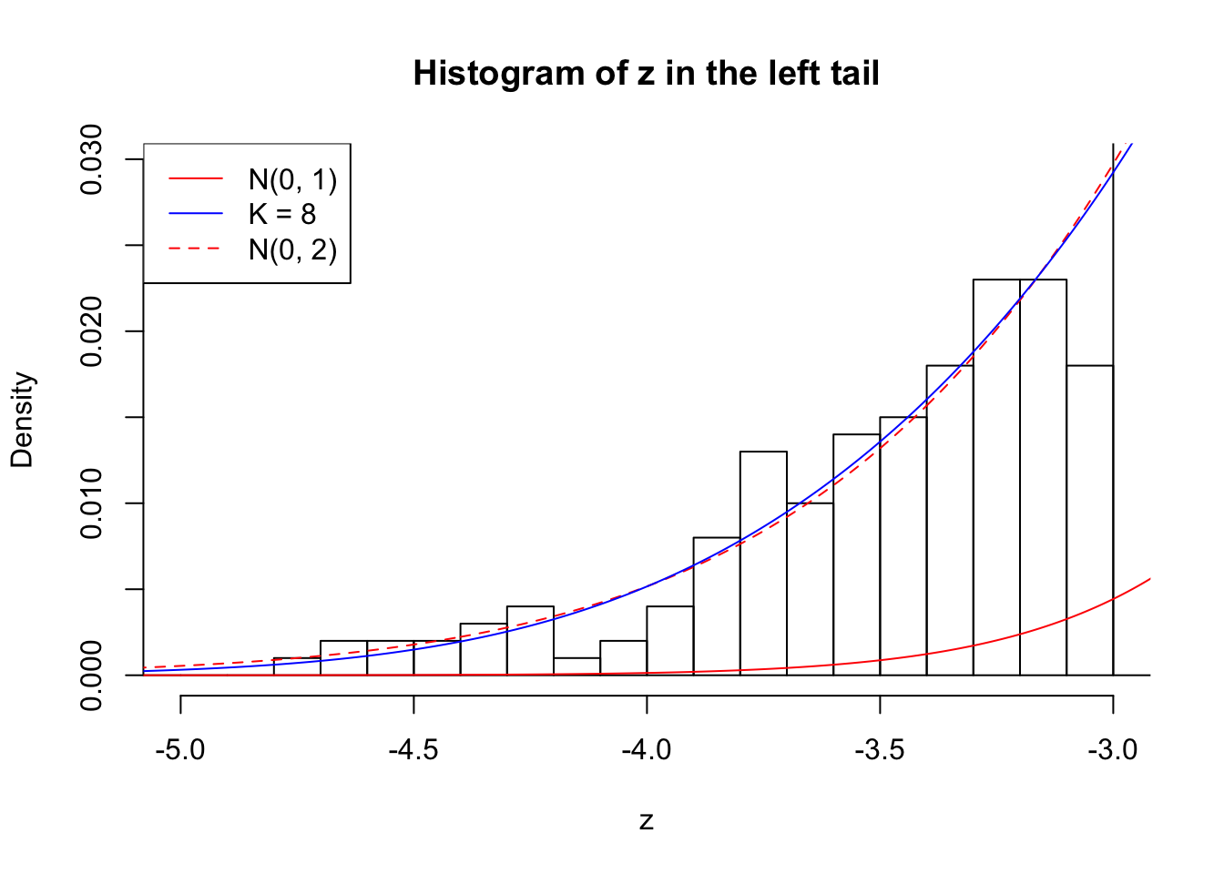

Zoom in to the right tail: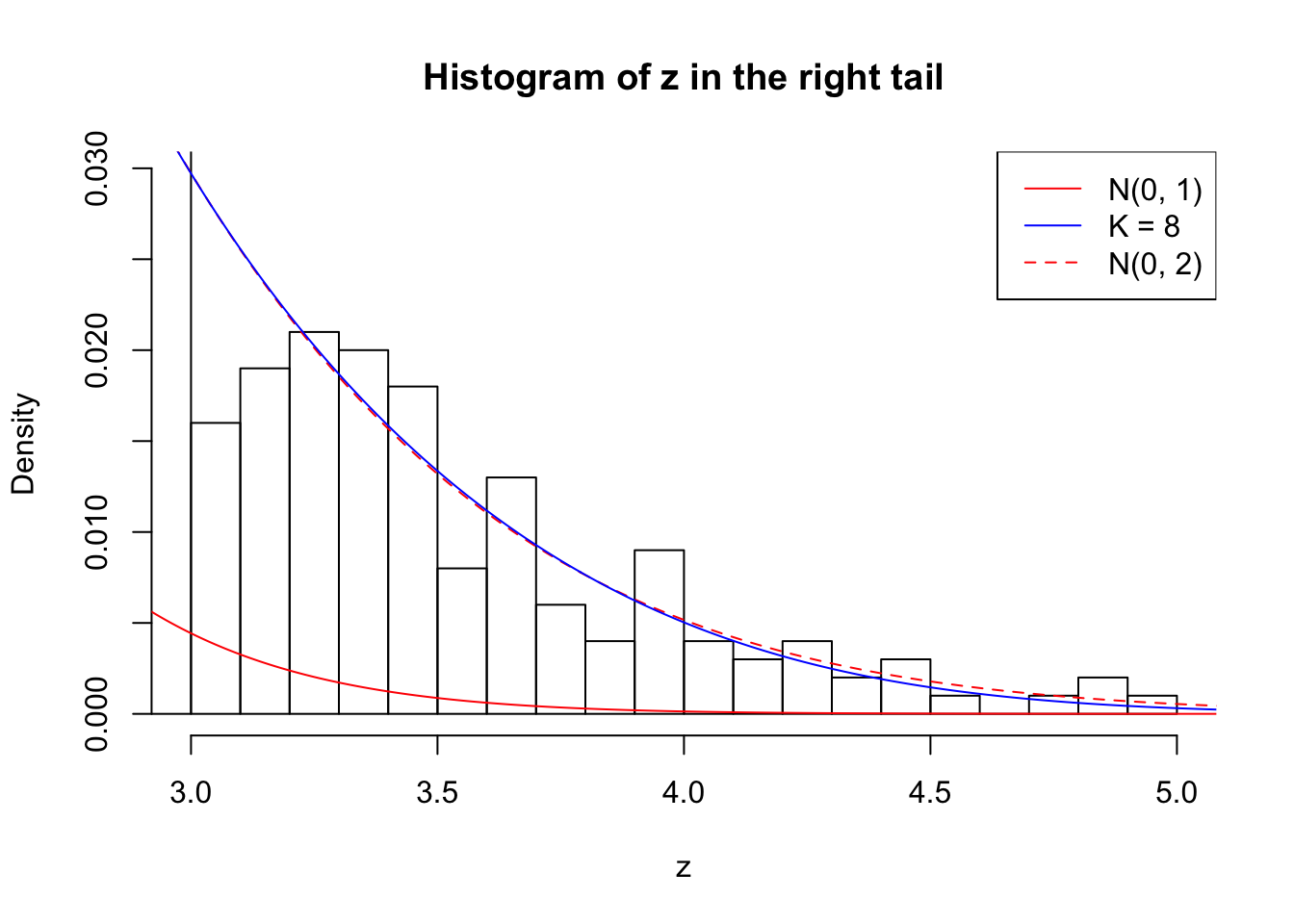

Example 3 : Number of Discoveries: 201 ; pihat0 = 0.3524008 
Log-likelihood with N(0, 2): -17627.66 
Log-likelihood with Gaussian Derivatives: -17623.26 
Log-likelihood ratio between true N(0, 2) and fitted Gaussian derivatives: -4.397359 
Normalized weights:
1 : 0.000611199281683122 ; 2 : 0.697833563596919 ; 3 : -9.24232505276873e-05 ; 4 : 0.593310577011007 ; 5 : 0.0690423192366928 ; 6 : 0.402719962212205 ; 7 : 0.0821756084741036 ; 8 : 0.137136244590824 ;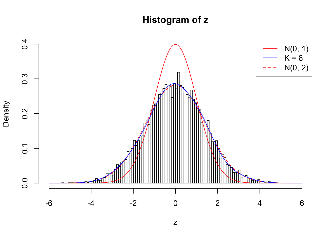

Zoom in to the left tail: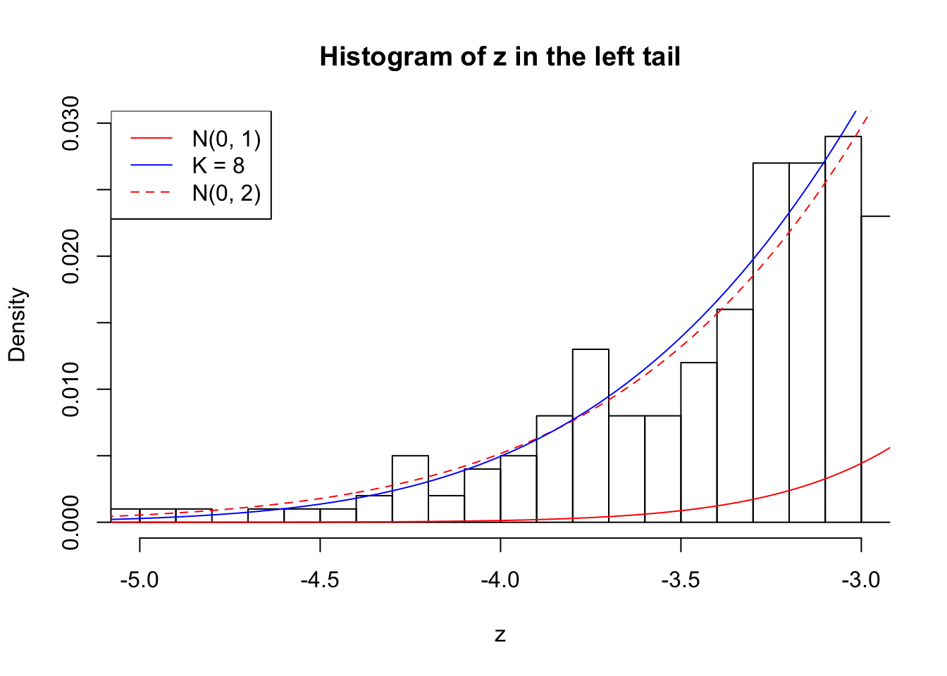

Zoom in to the right tail: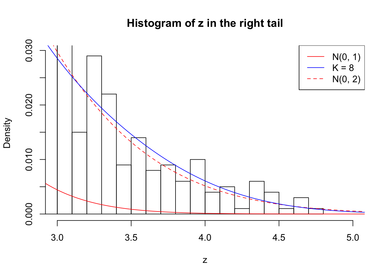

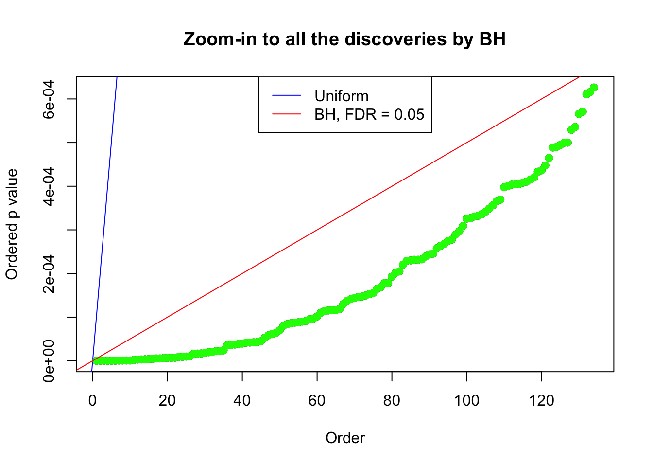
Example 4 : Number of Discoveries: 134 ; pihat0 = 0.3039997 
Log-likelihood with N(0, 2): -17572.28 
Log-likelihood with Gaussian Derivatives: -17589.35 
Log-likelihood ratio between true N(0, 2) and fitted Gaussian derivatives: 17.07424 
Normalized weights:
1 : -0.00303021567753385 ; 2 : 0.667140676046508 ; 3 : -0.00744442518950379 ; 4 : 0.4335954662891 ; 5 : 0.00652056989516479 ; 6 : 0.163579551221406 ; 7 : 0.0434395776822699 ;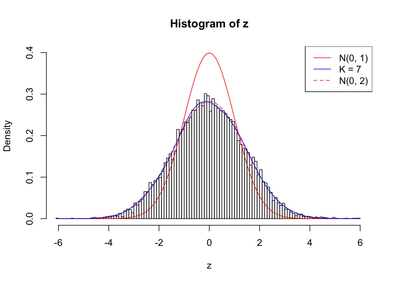

Zoom in to the left tail: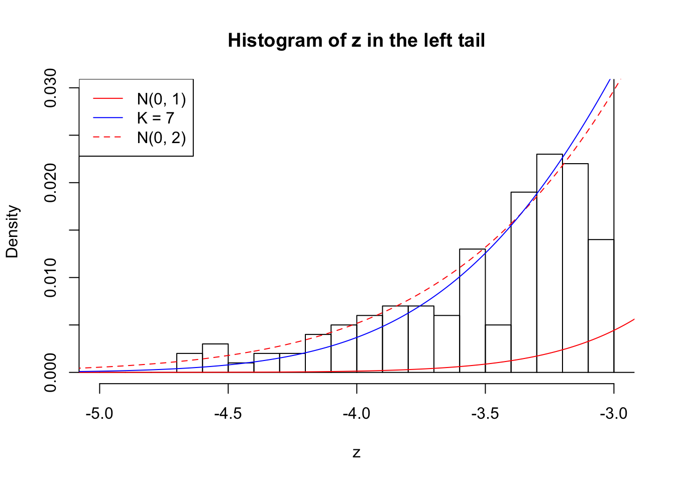

Zoom in to the right tail: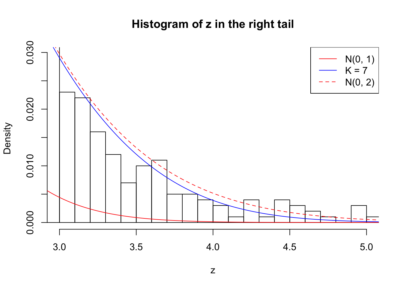

Example 5 : Number of Discoveries: 201 ; pihat0 = 0.3864133 
Log-likelihood with N(0, 2): -17602.8 
Log-likelihood with Gaussian Derivatives: -17607.36 
Log-likelihood ratio between true N(0, 2) and fitted Gaussian derivatives: 4.565327 
Normalized weights:
1 : -0.0149505230188178 ; 2 : 0.681006373173563 ; 3 : -0.029408092099831 ; 4 : 0.526597120212115 ; 5 : -0.0649823448928799 ; 6 : 0.248323484516014 ; 7 : -0.077154633635199 ;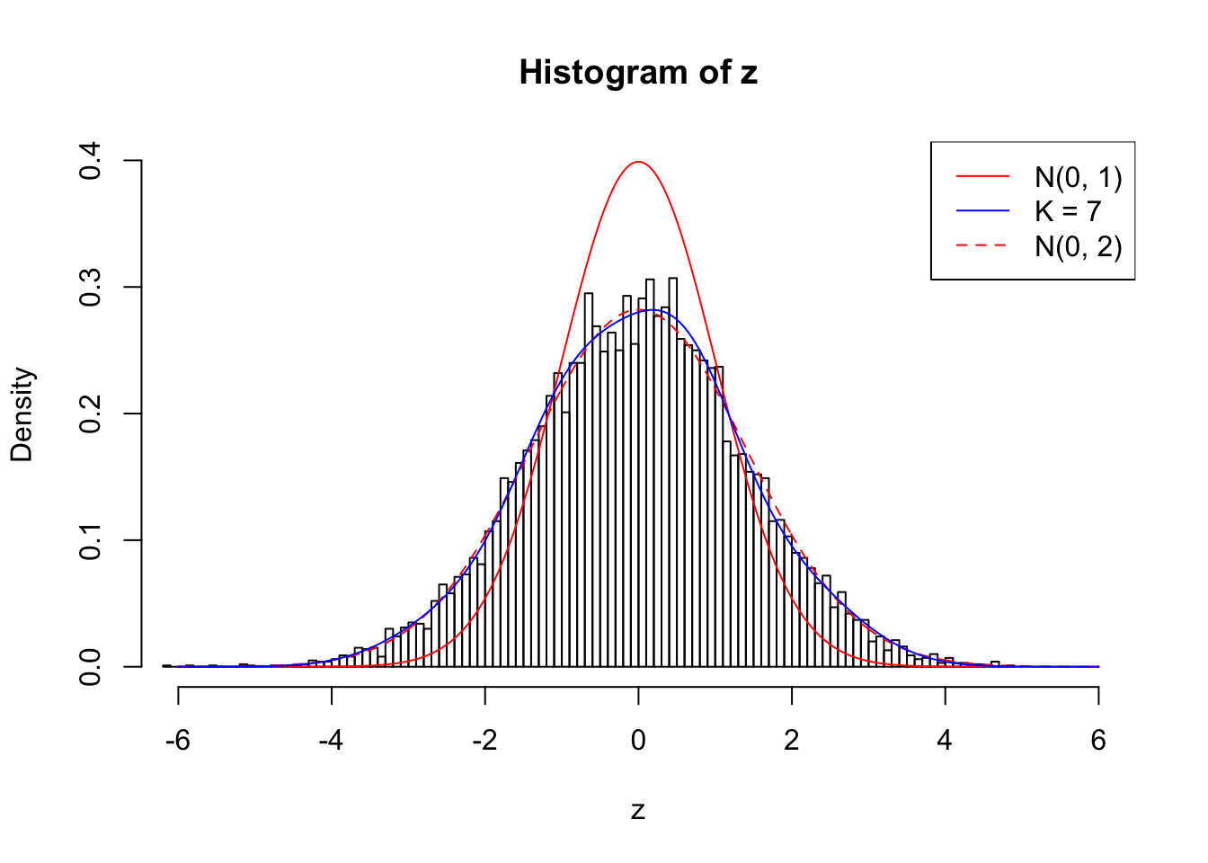

Zoom in to the left tail: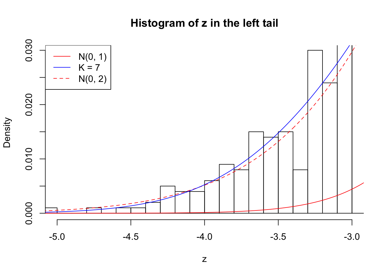

Zoom in to the right tail: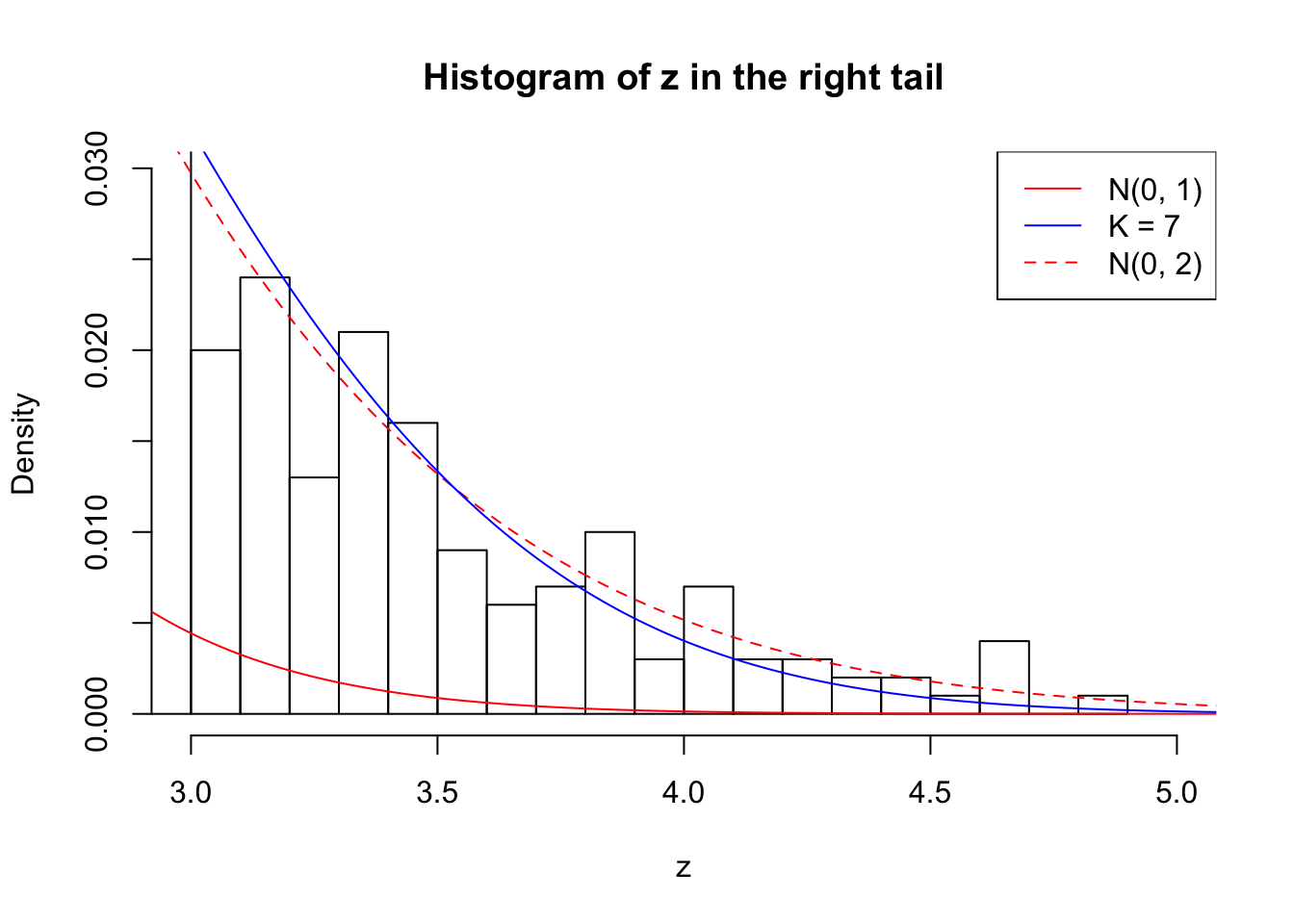

Session information

sessionInfo()

R version 3.4.3 (2017-11-30)
Platform: x86_64-apple-darwin15.6.0 (64-bit)
Running under: macOS High Sierra 10.13.2

Matrix products: default
BLAS: /Library/Frameworks/R.framework/Versions/3.4/Resources/lib/libRblas.0.dylib
LAPACK: /Library/Frameworks/R.framework/Versions/3.4/Resources/lib/libRlapack.dylib

locale:
[1] en_US.UTF-8/en_US.UTF-8/en_US.UTF-8/C/en_US.UTF-8/en_US.UTF-8

attached base packages:
[1] stats     graphics  grDevices utils     datasets  methods   base     

loaded via a namespace (and not attached):
 [1] compiler_3.4.3  backports_1.1.2 magrittr_1.5    rprojroot_1.3-1
 [5] tools_3.4.3     htmltools_0.3.6 yaml_2.1.16     Rcpp_0.12.14   
 [9] stringi_1.1.6   rmarkdown_1.8   knitr_1.17      git2r_0.20.0   
[13] stringr_1.2.0   digest_0.6.13   evaluate_0.10.1