Diagnostic Plots for ASH on Correlated Null
Lei Sun
2017-04-18
Last updated: 2017-12-21
Code version: 6e42447
Correlation makes ASH fit less well
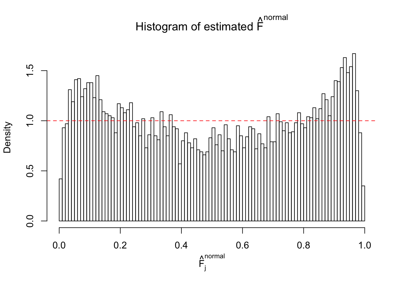
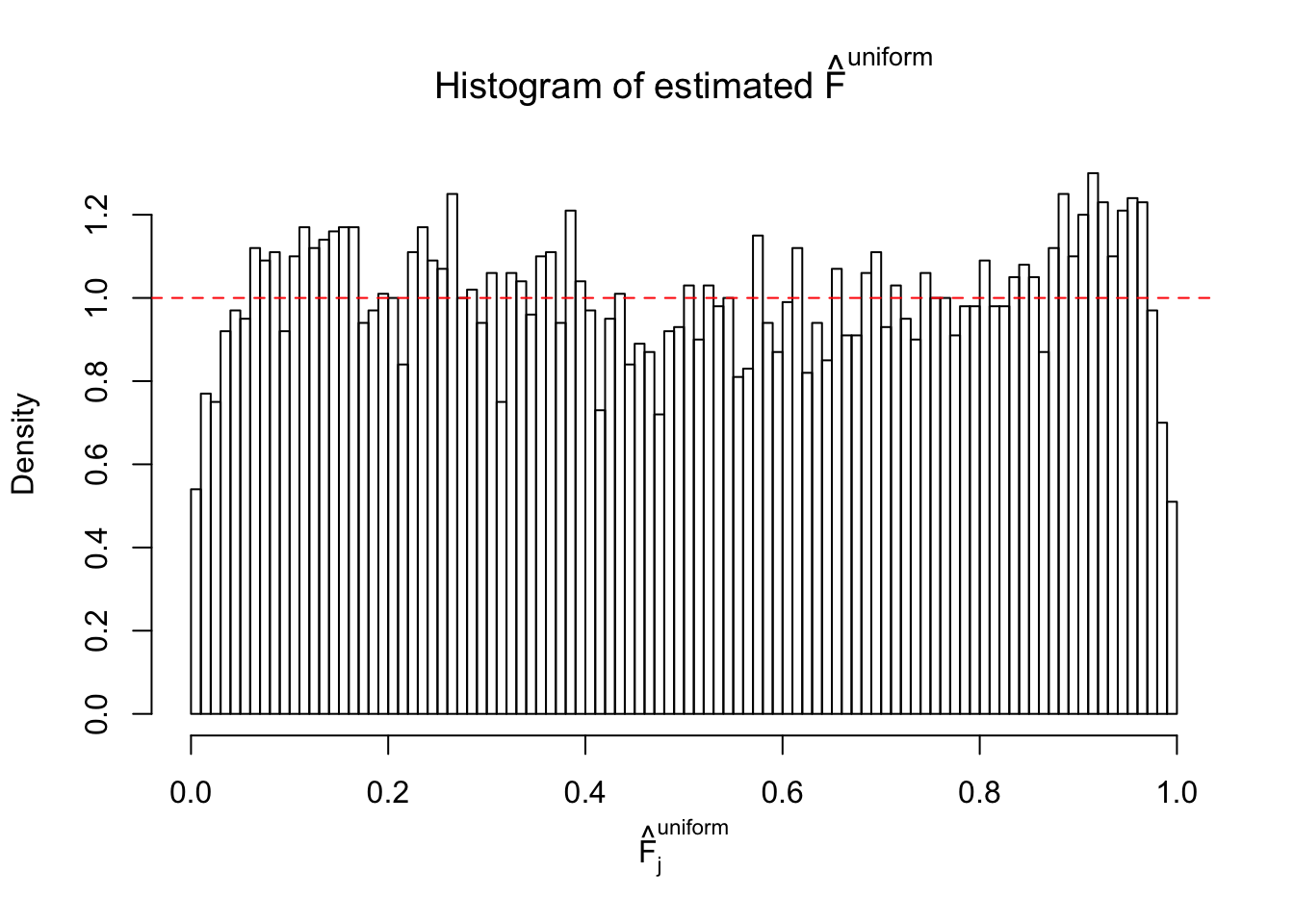
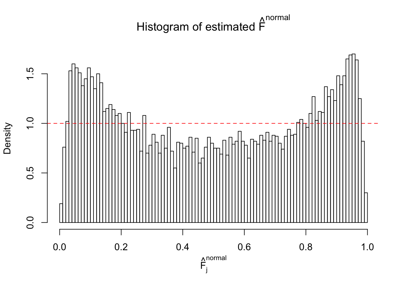
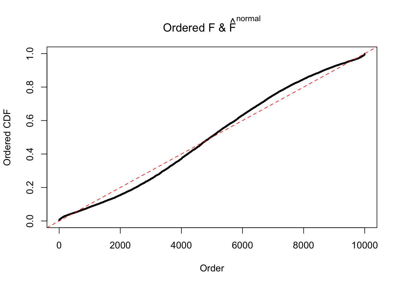
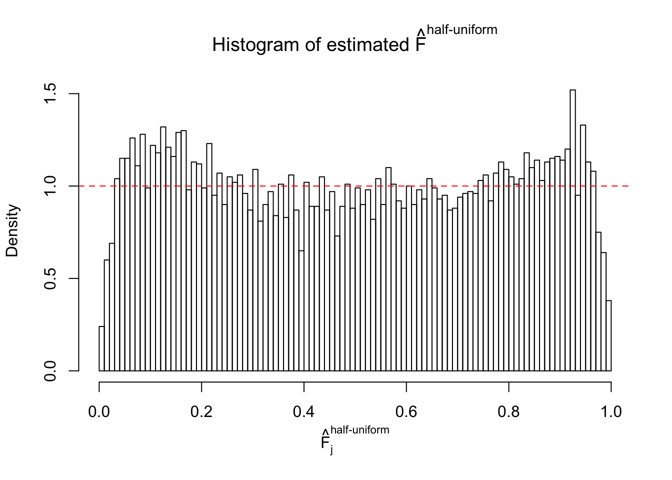
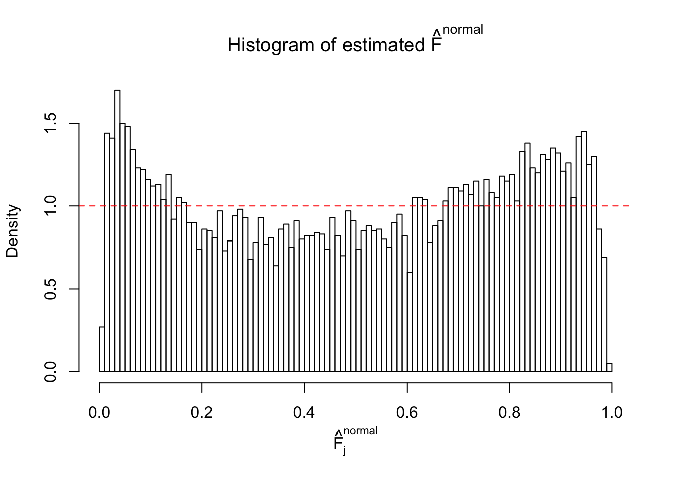
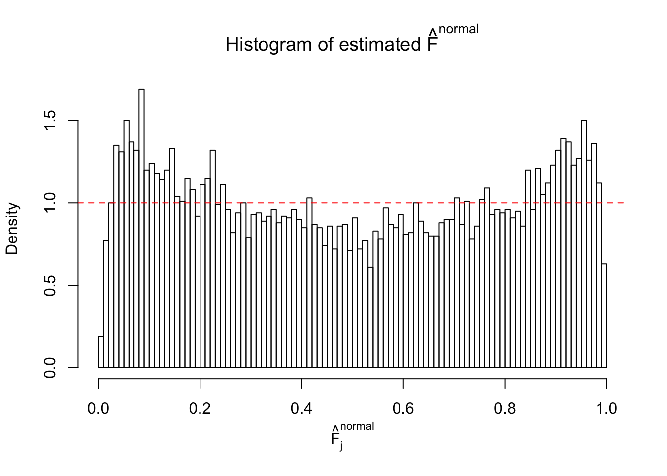
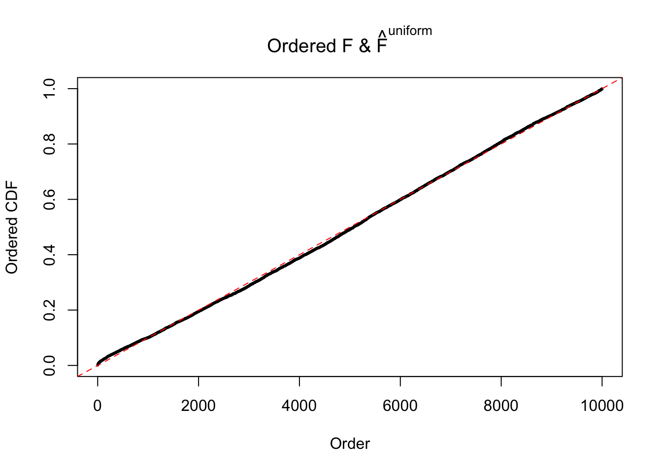
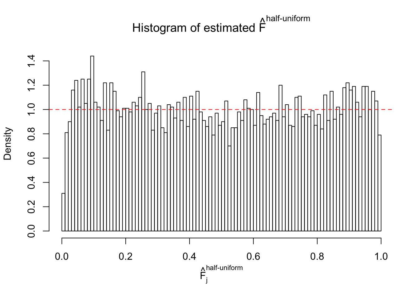
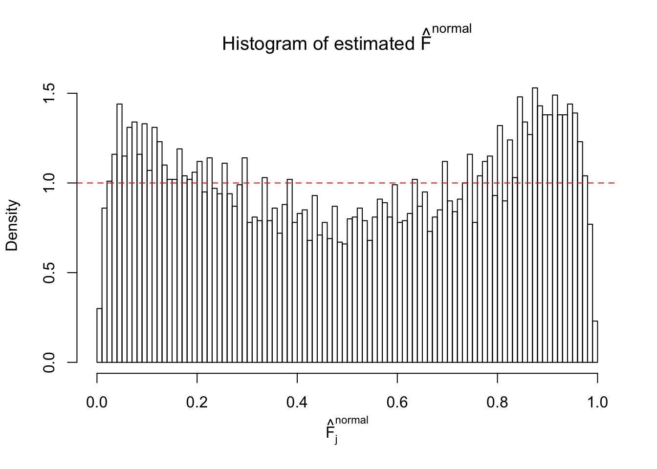
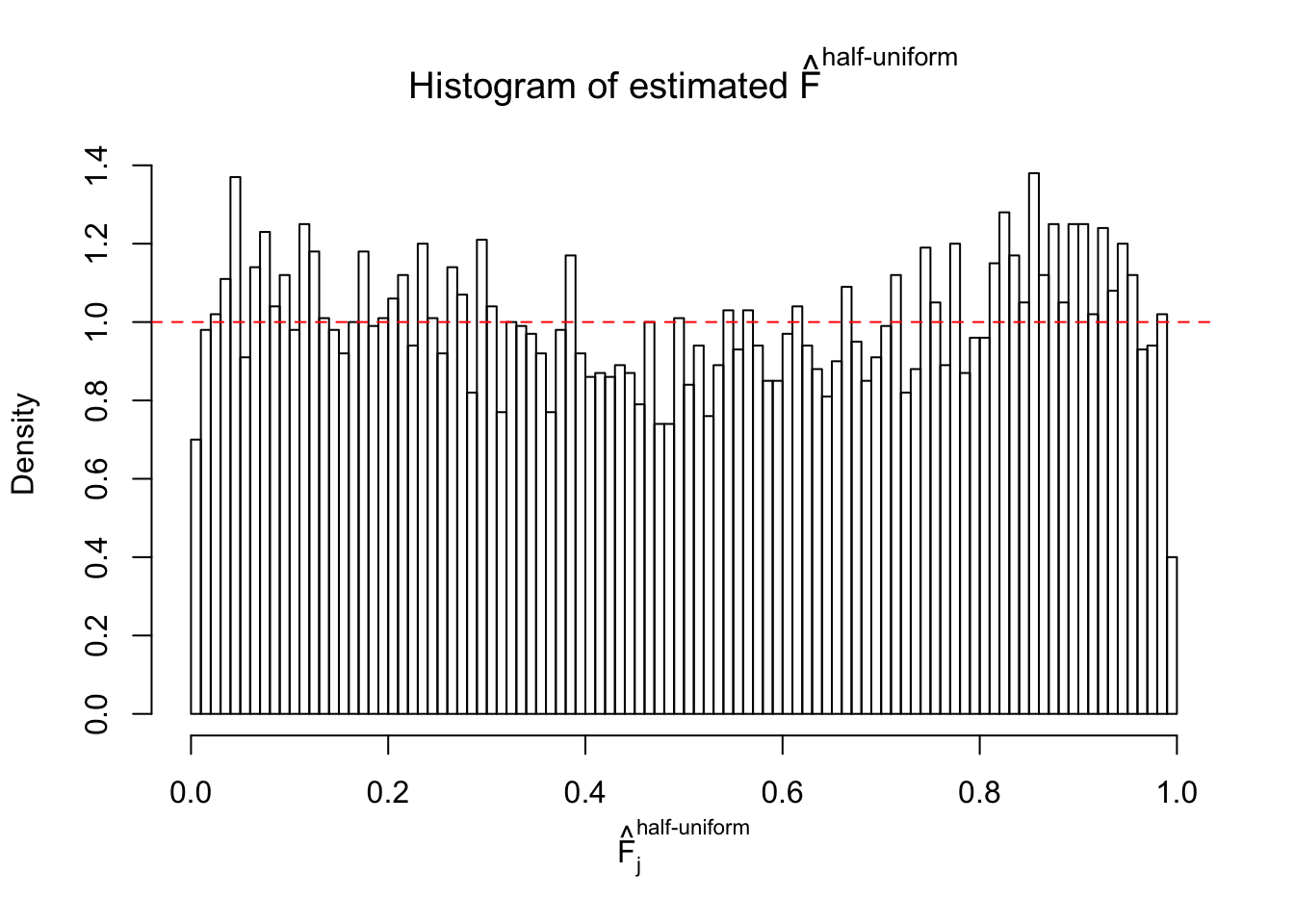
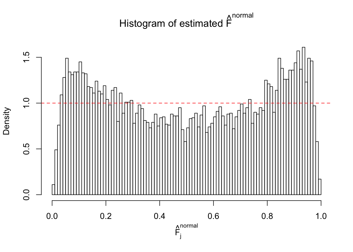
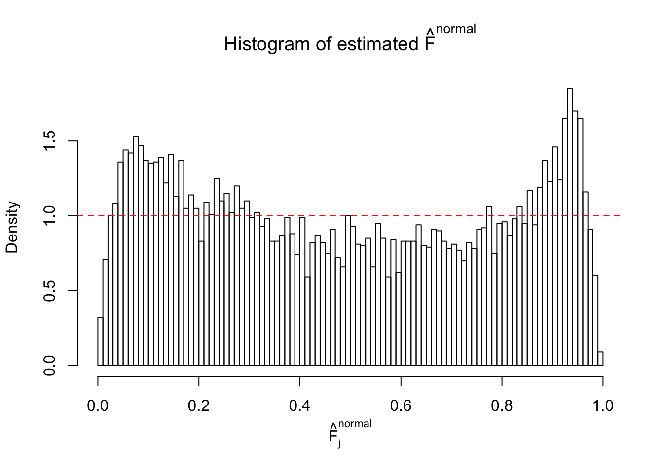
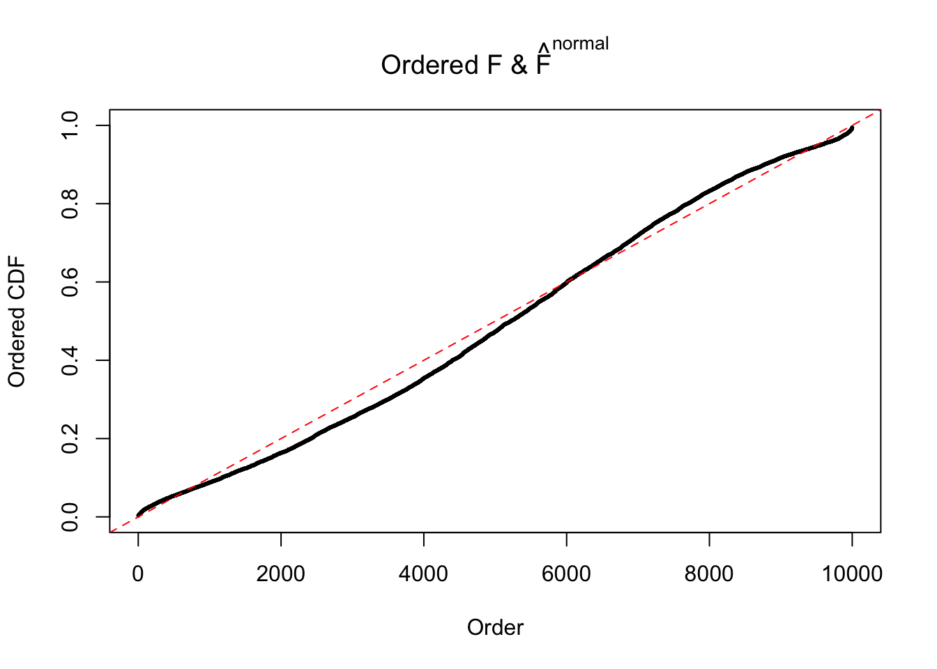
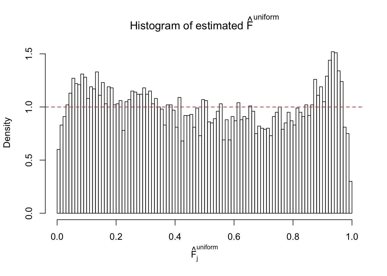
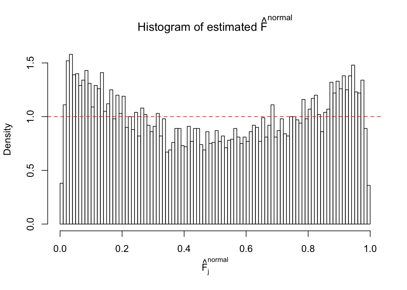
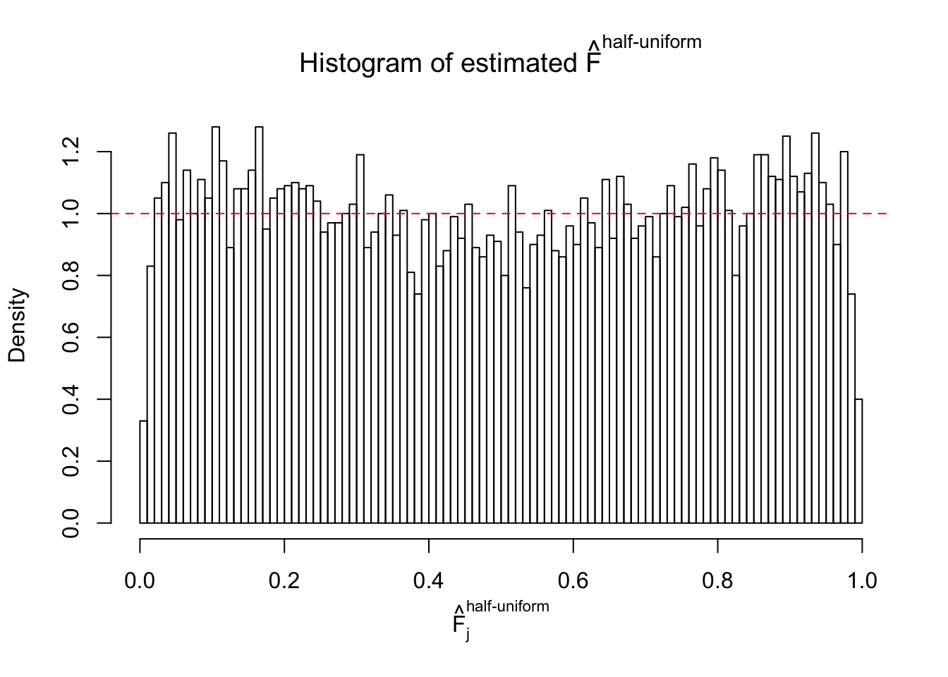
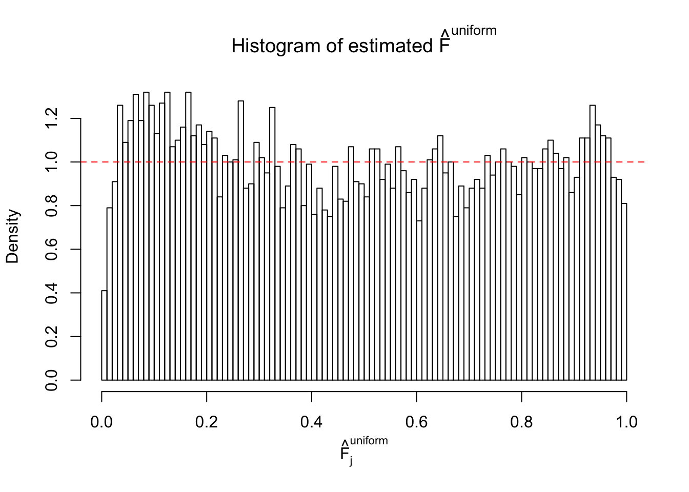
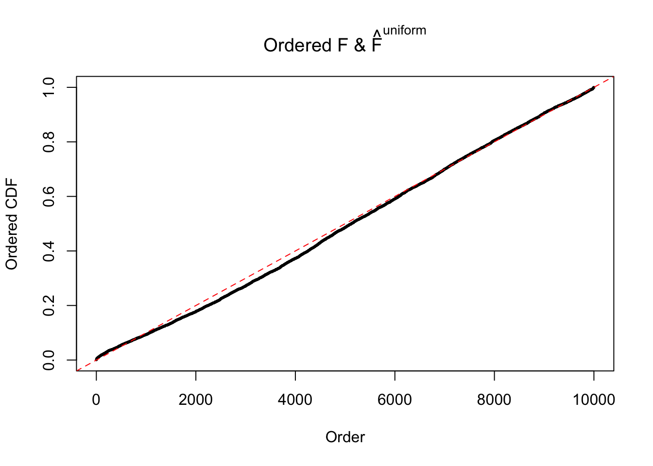
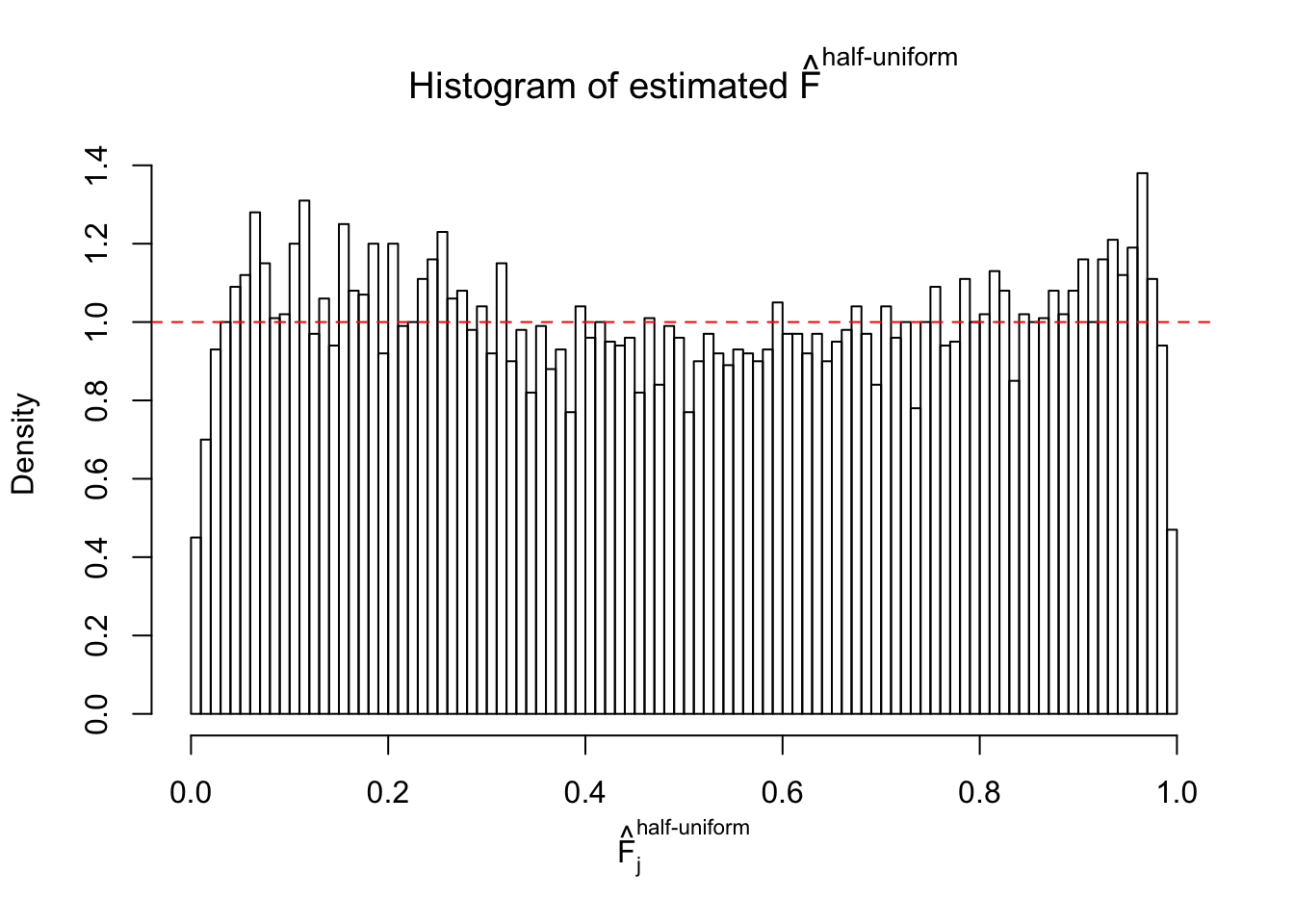
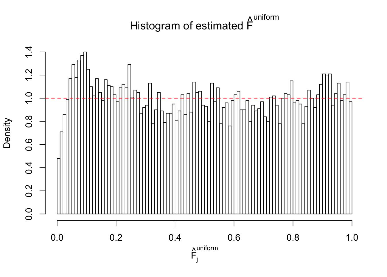
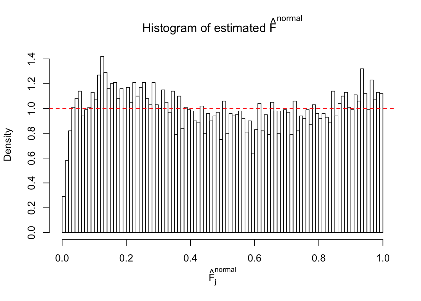
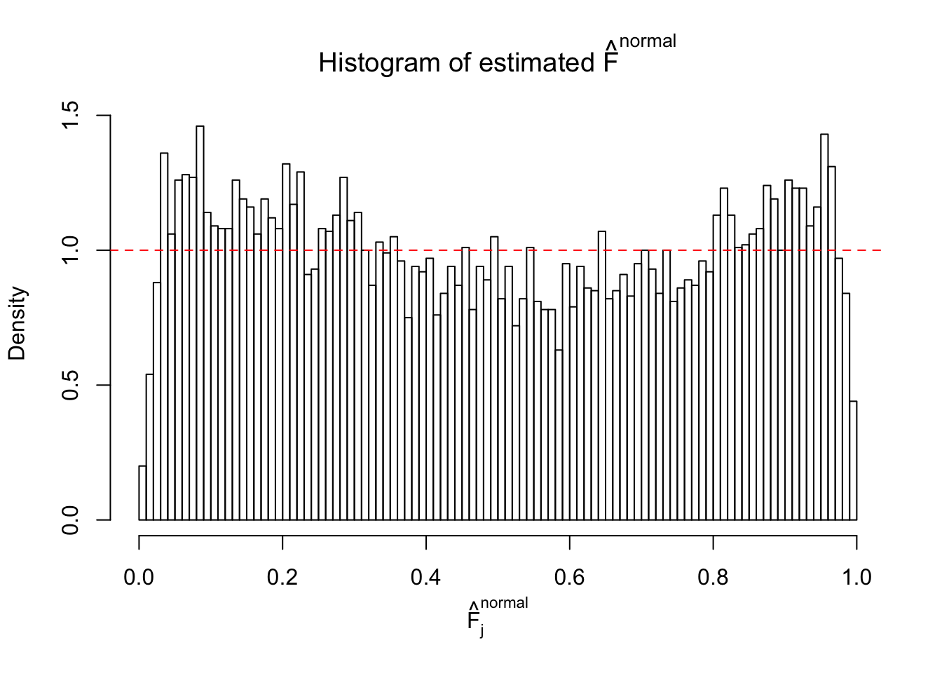
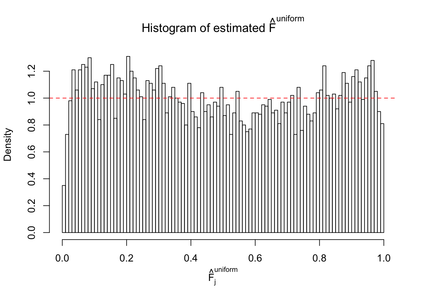
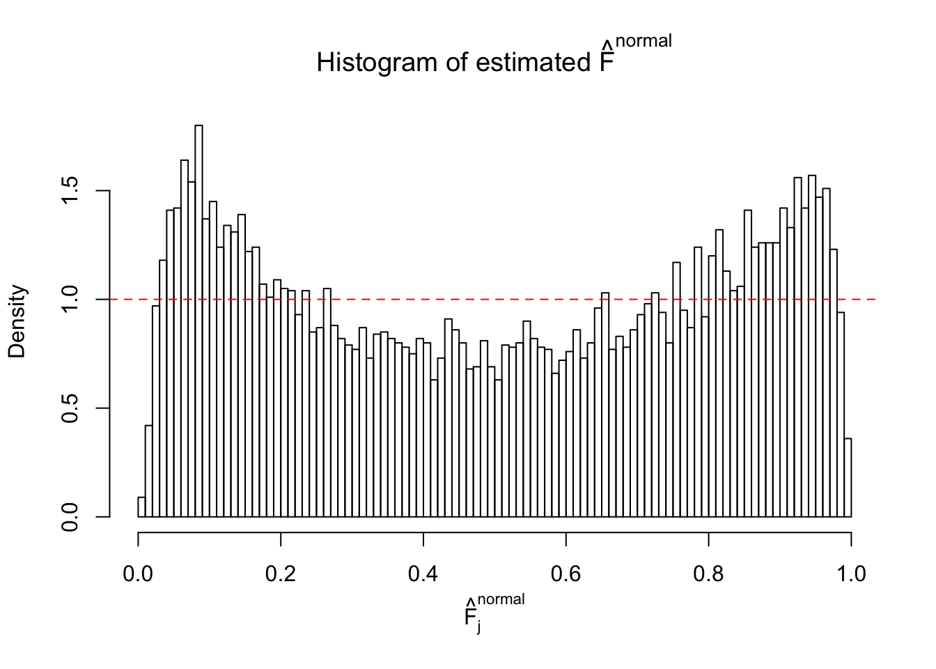
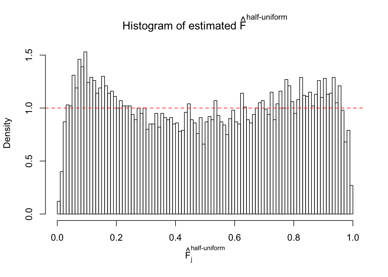
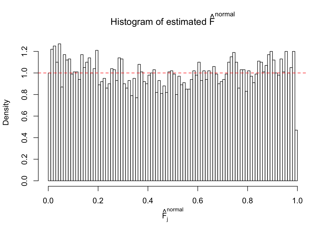
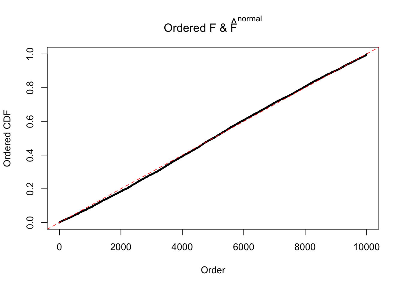
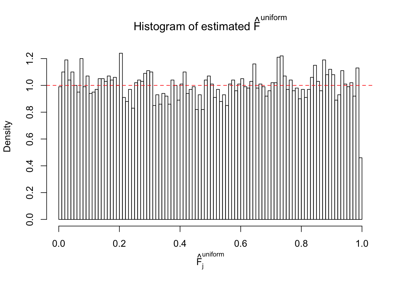
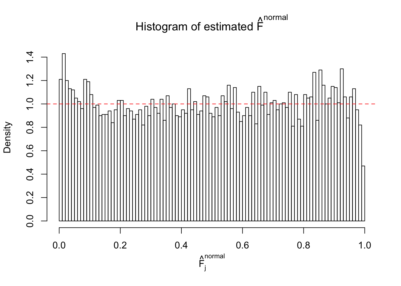
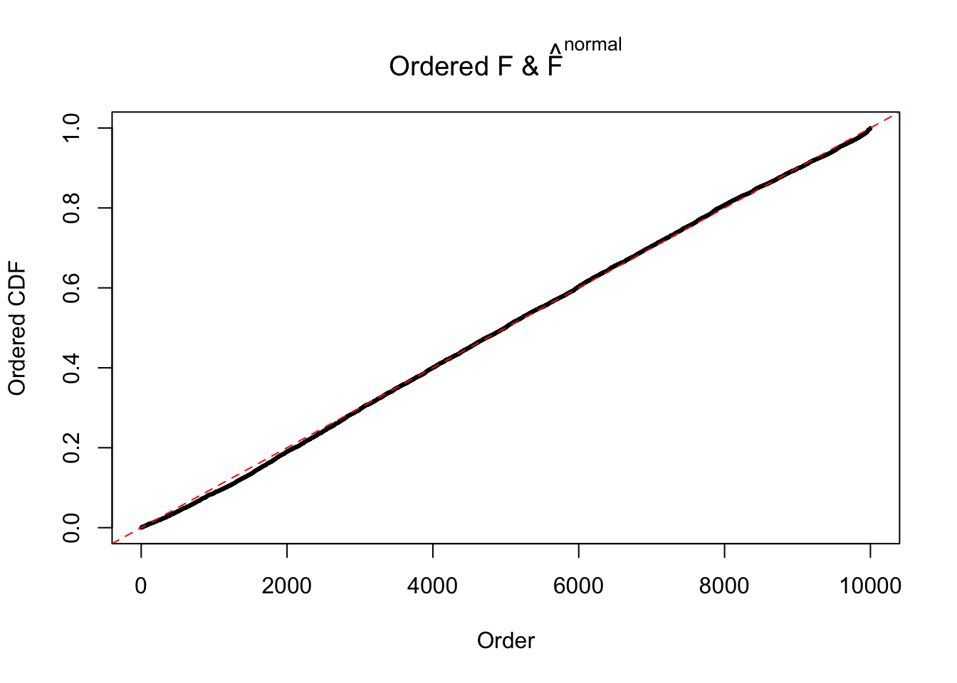
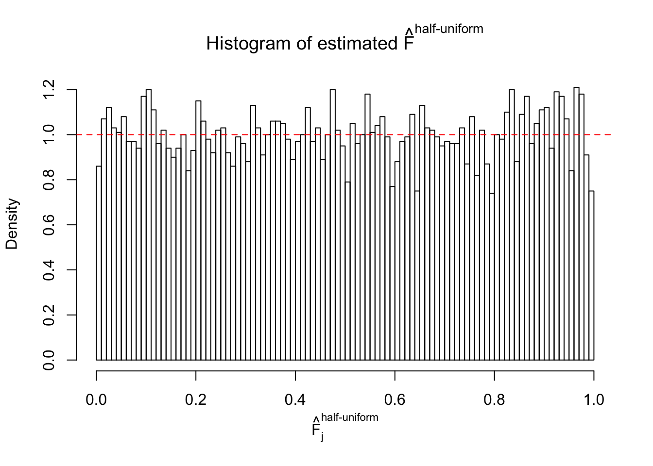
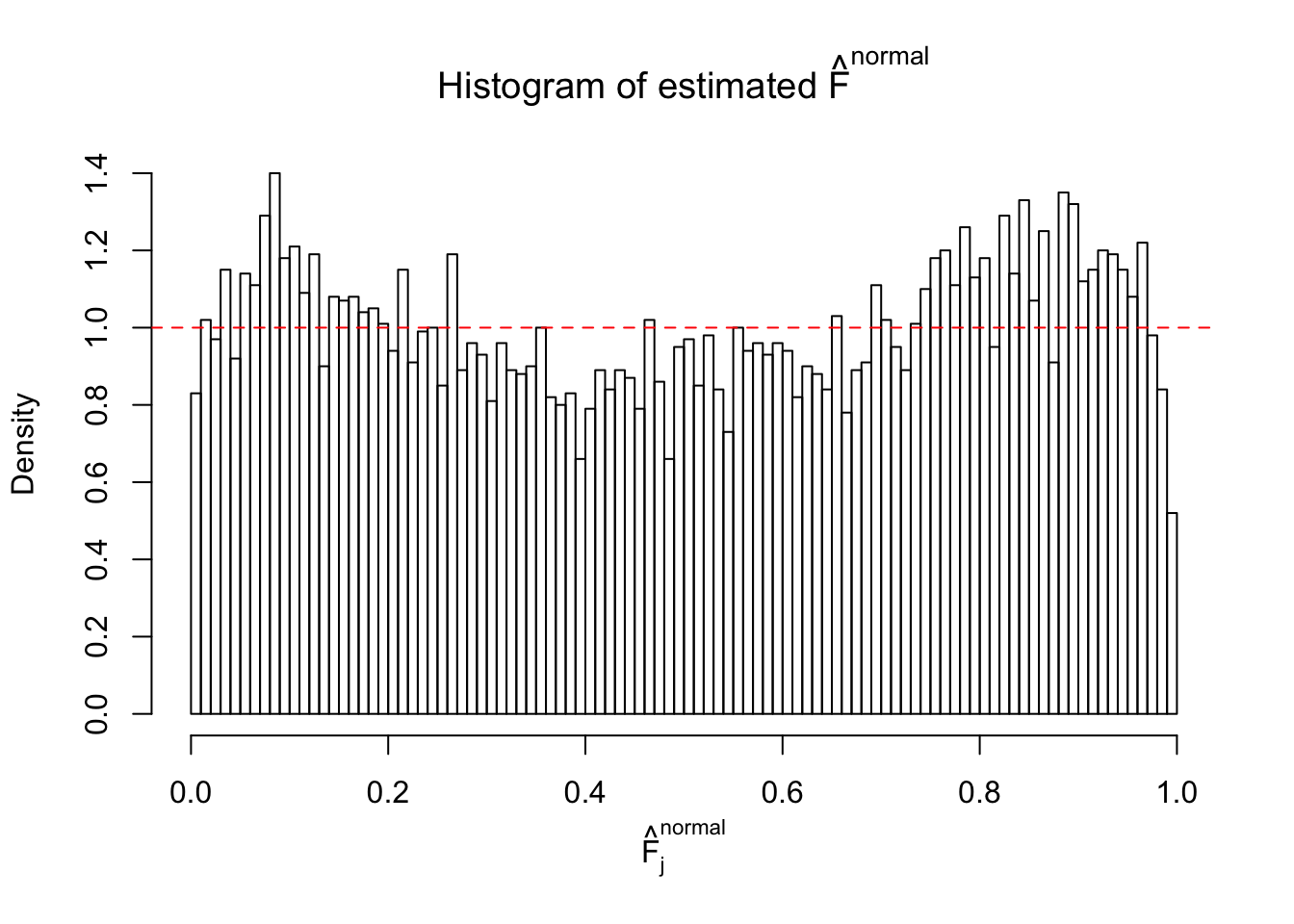
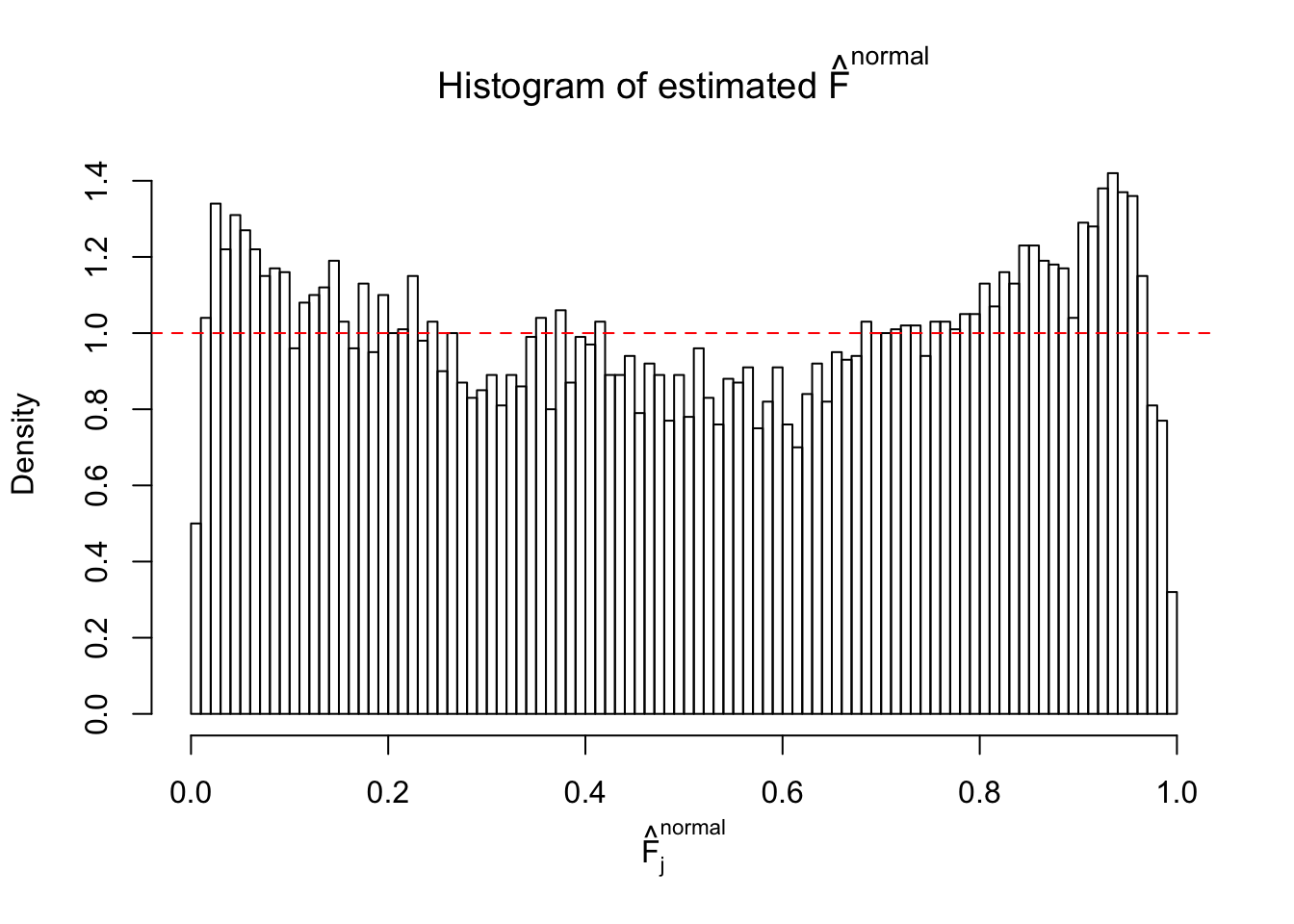
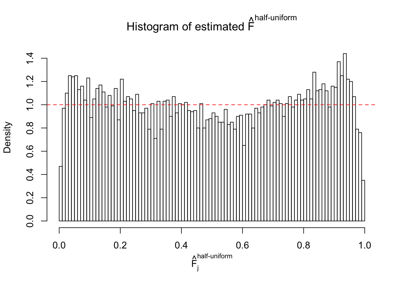
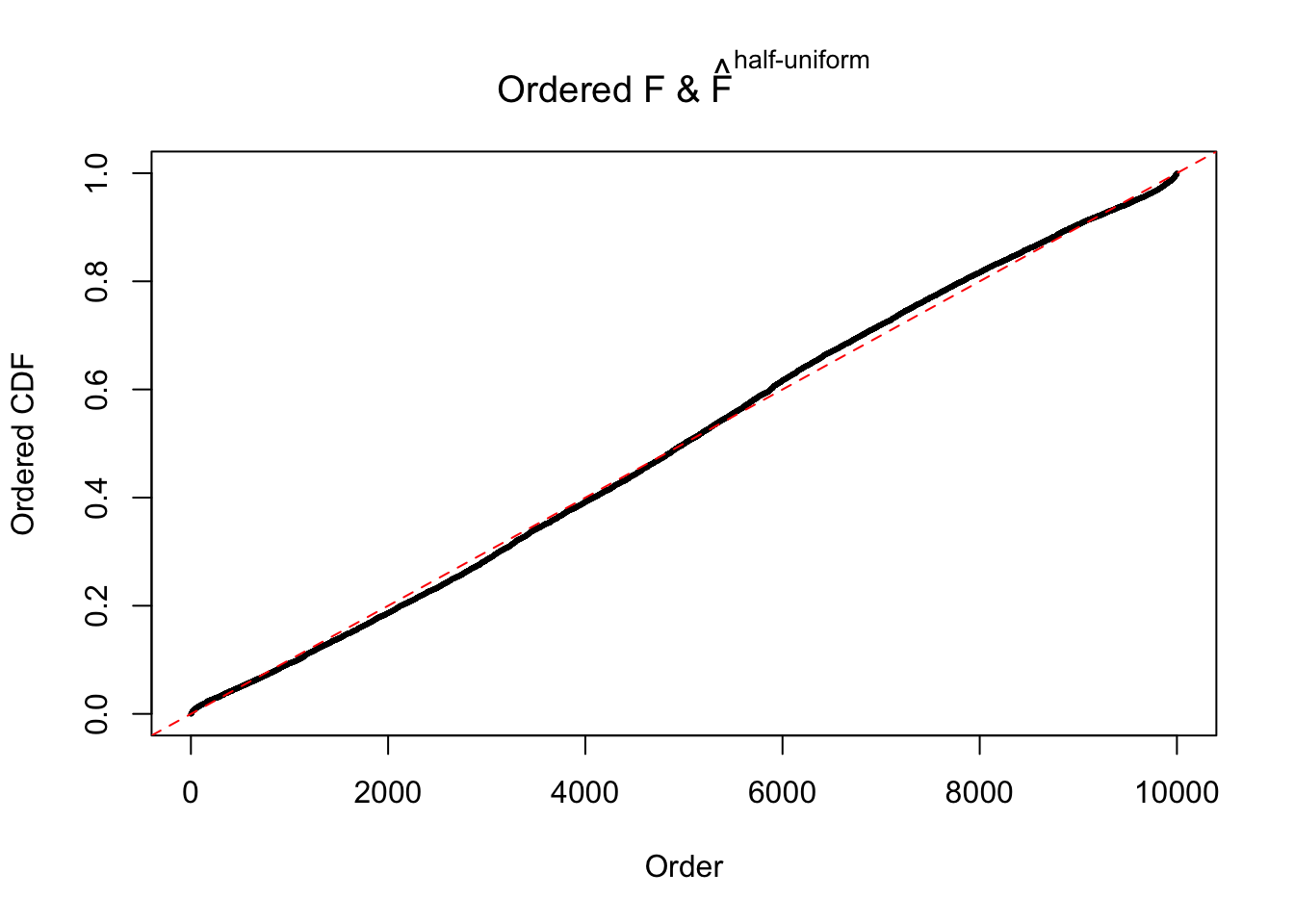
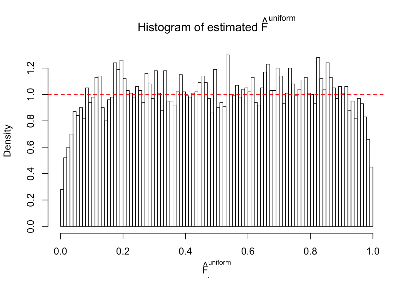
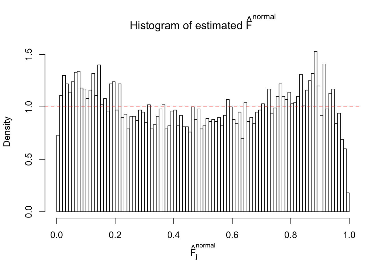
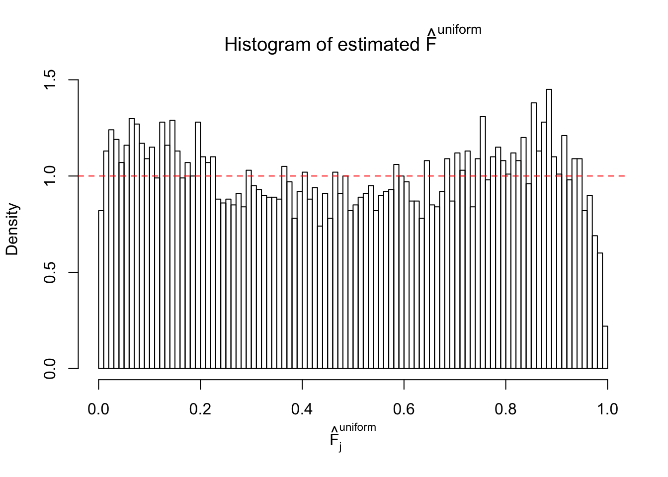
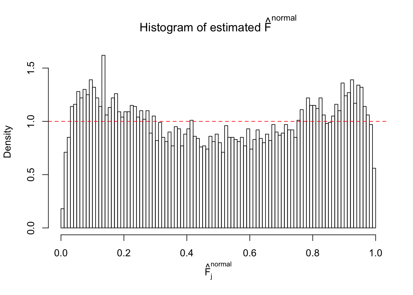
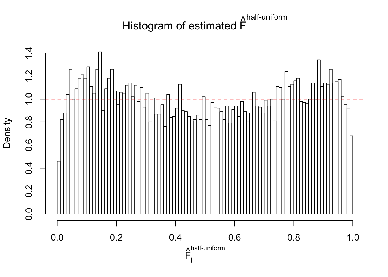
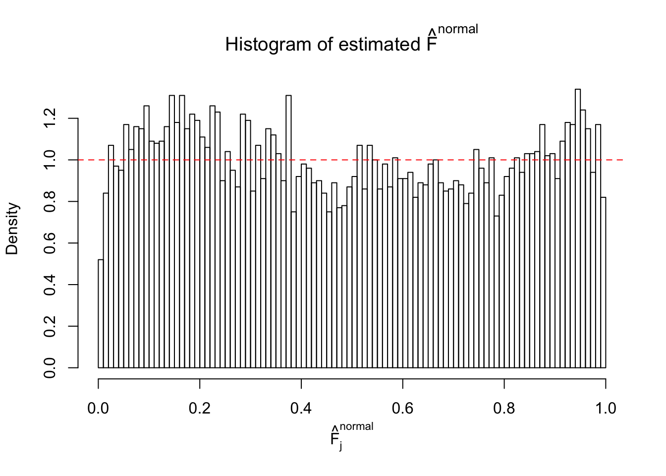
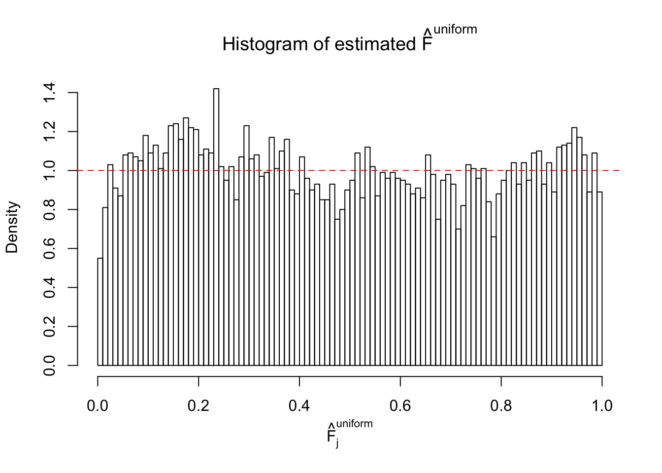
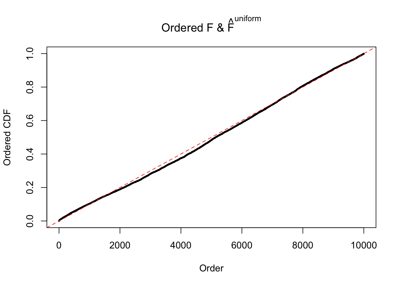
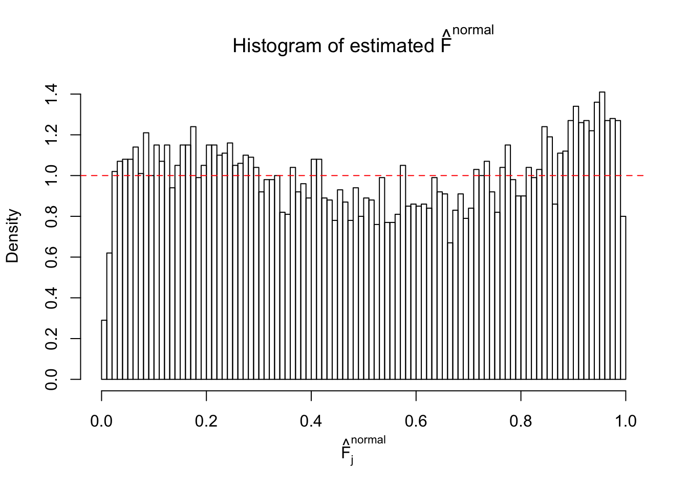
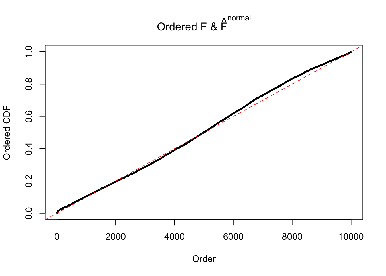
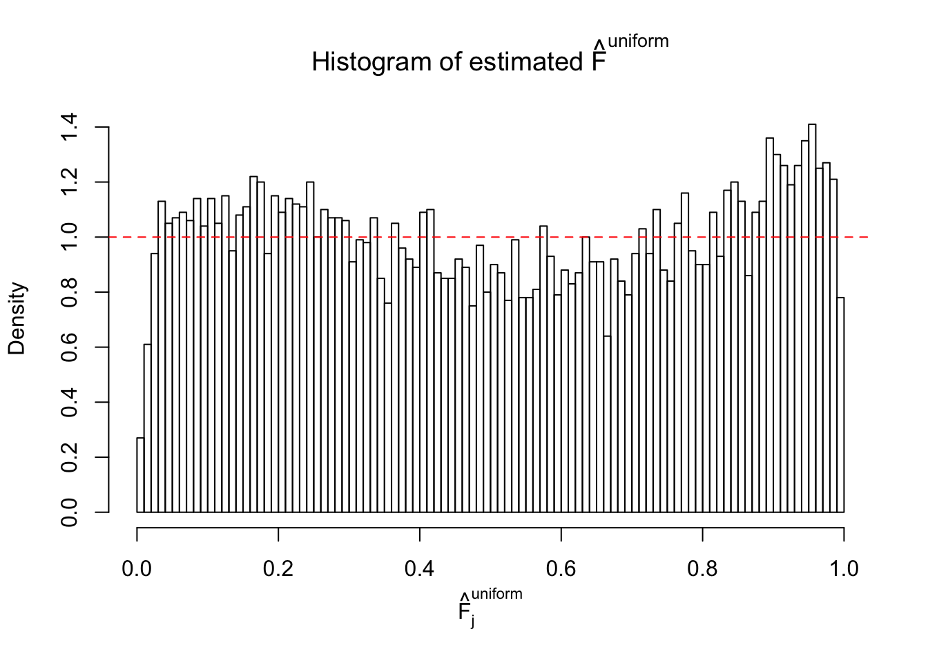
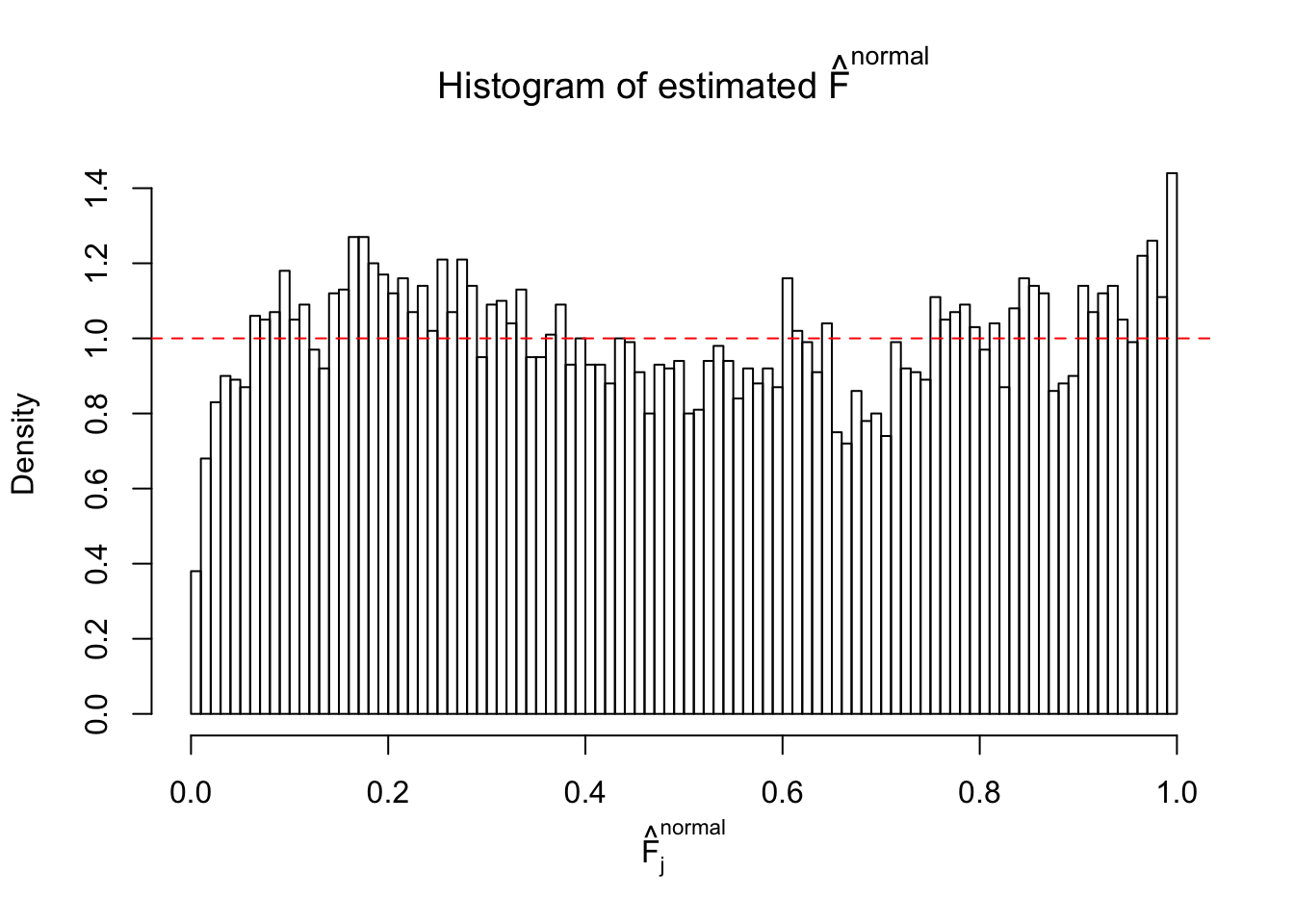
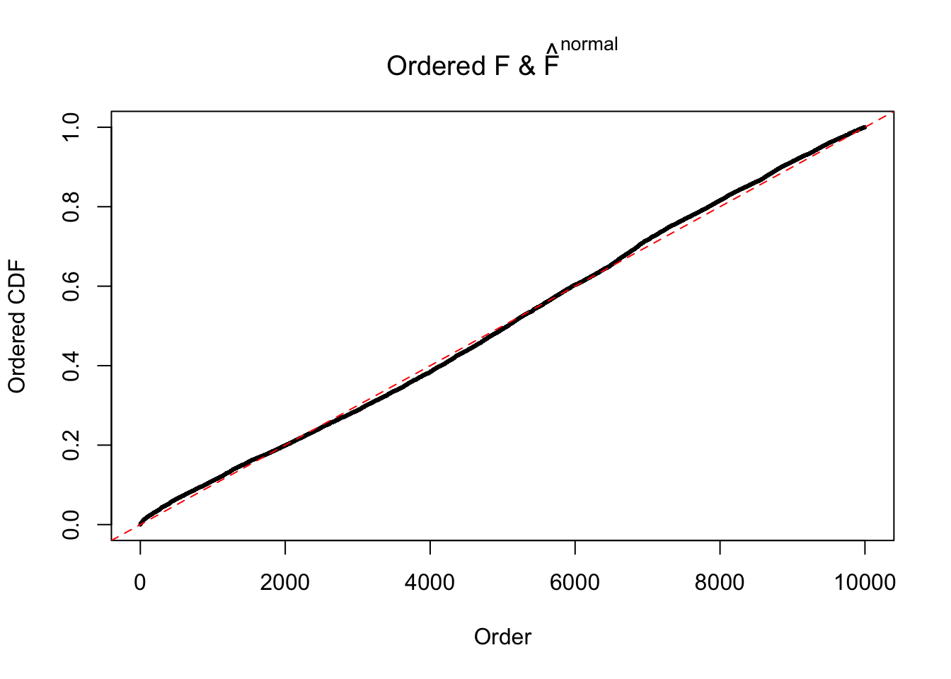
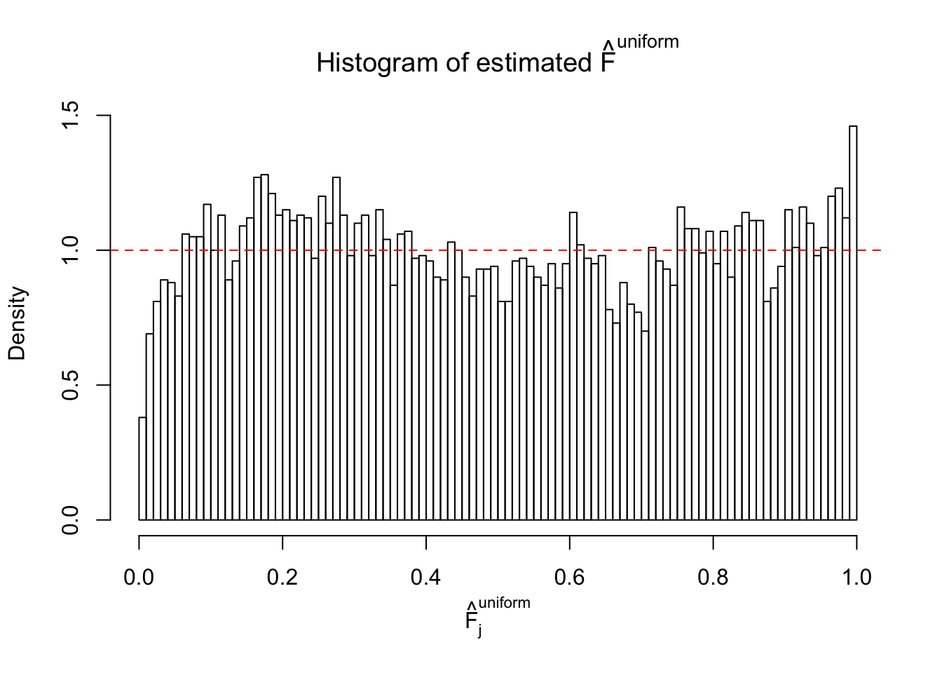
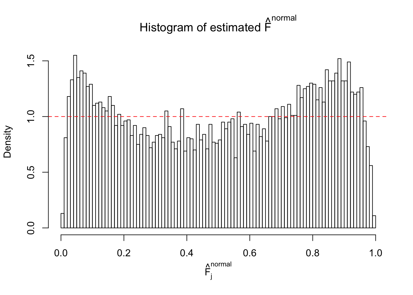
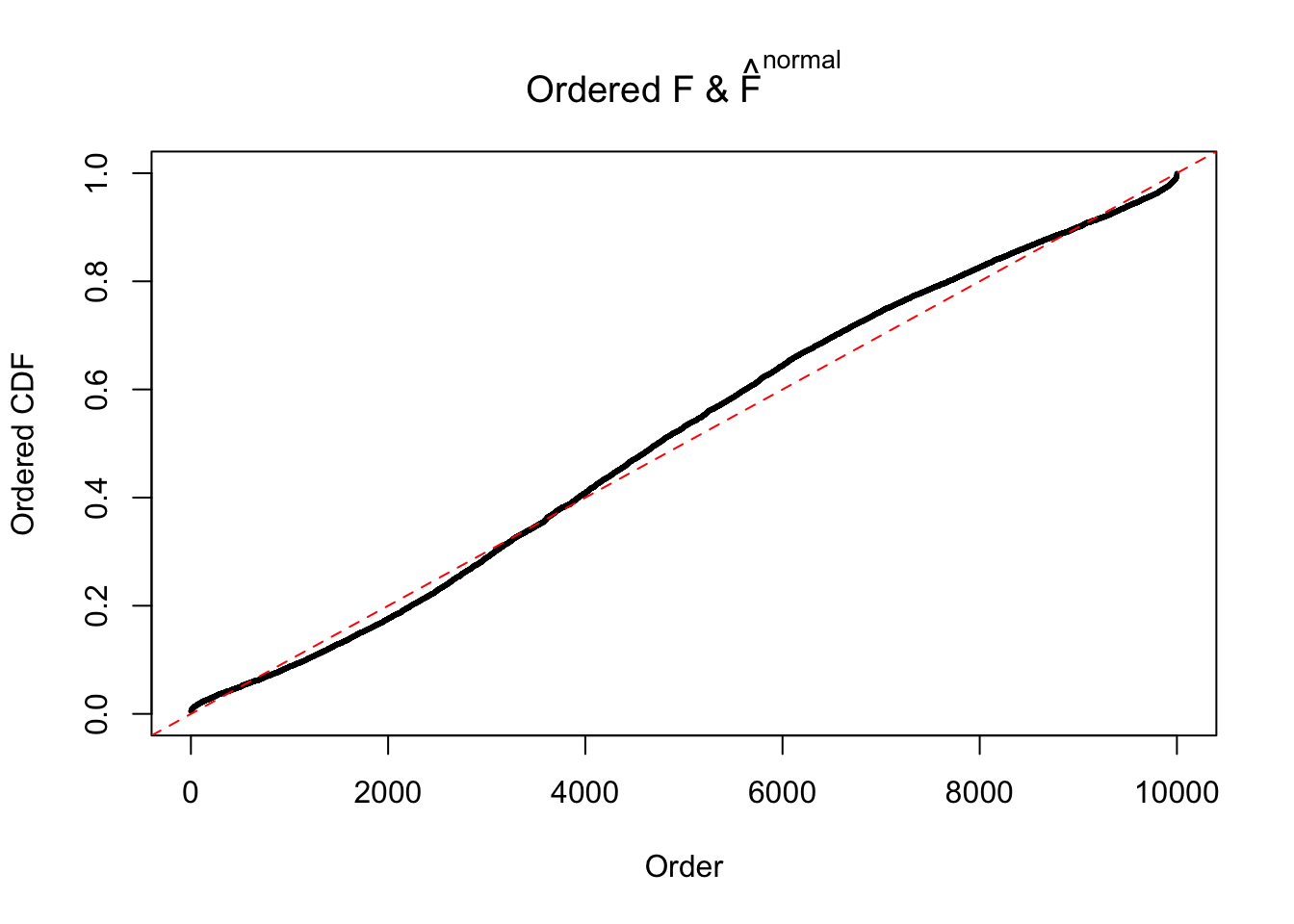
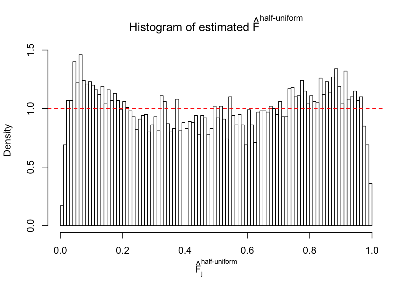
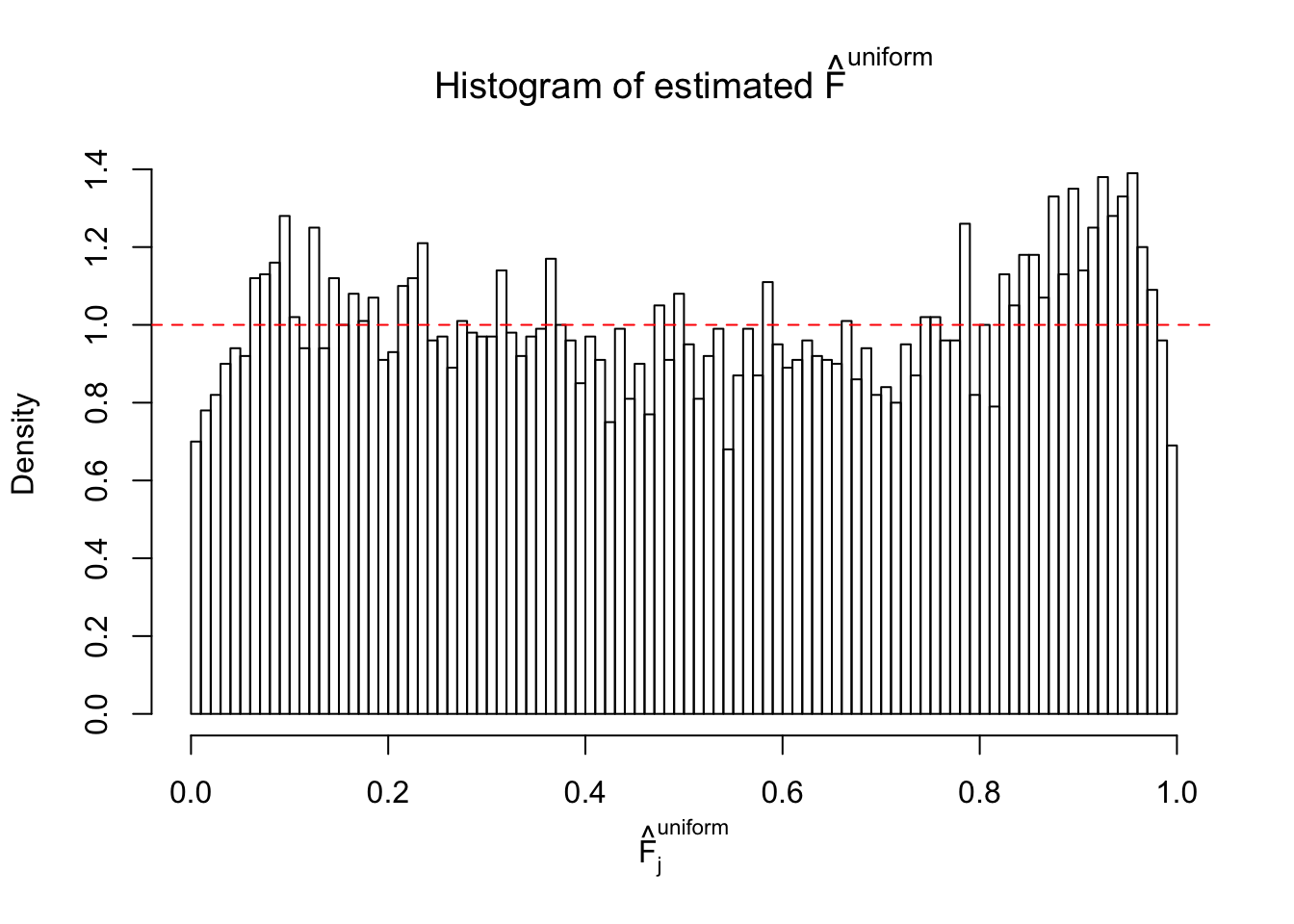
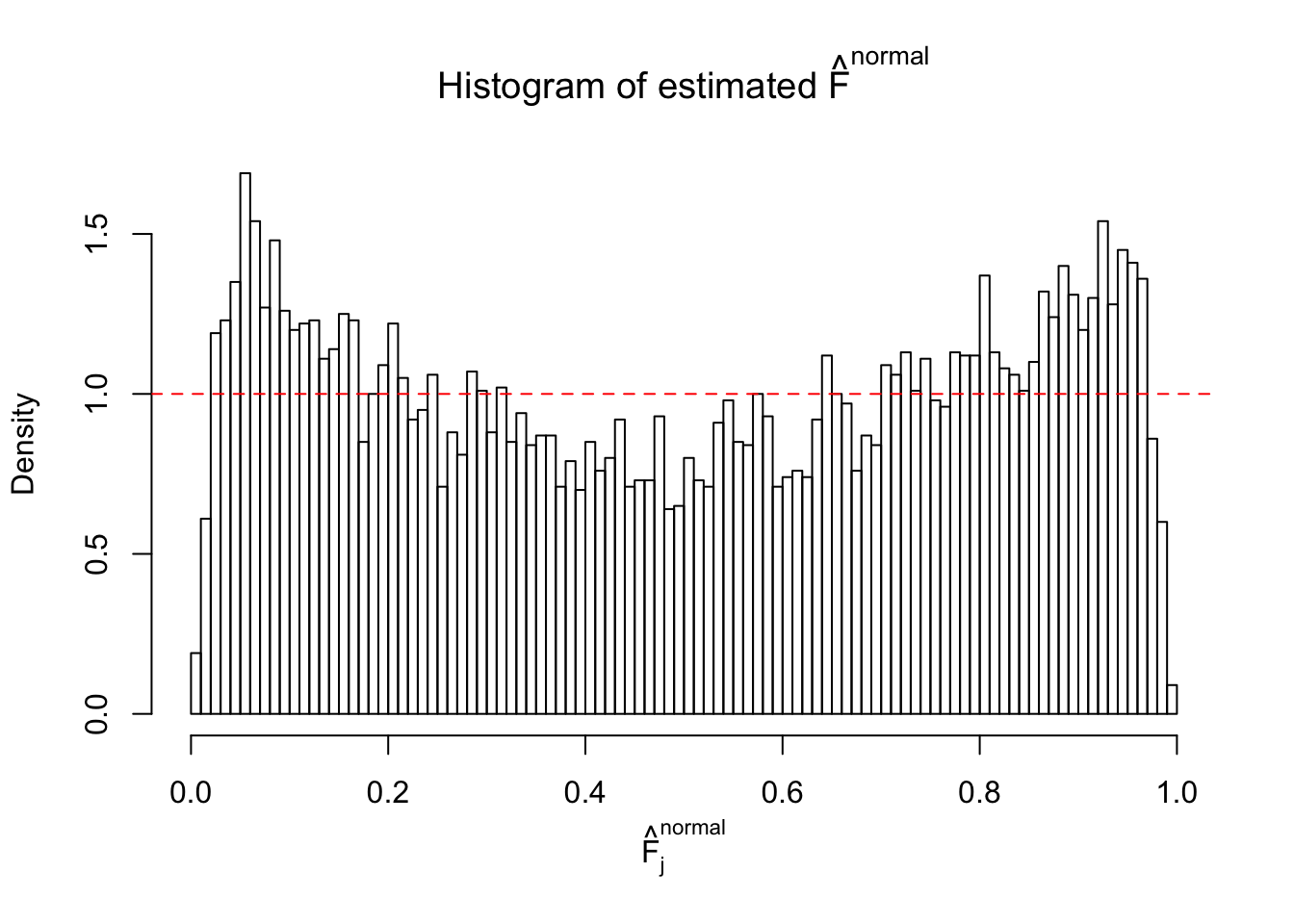
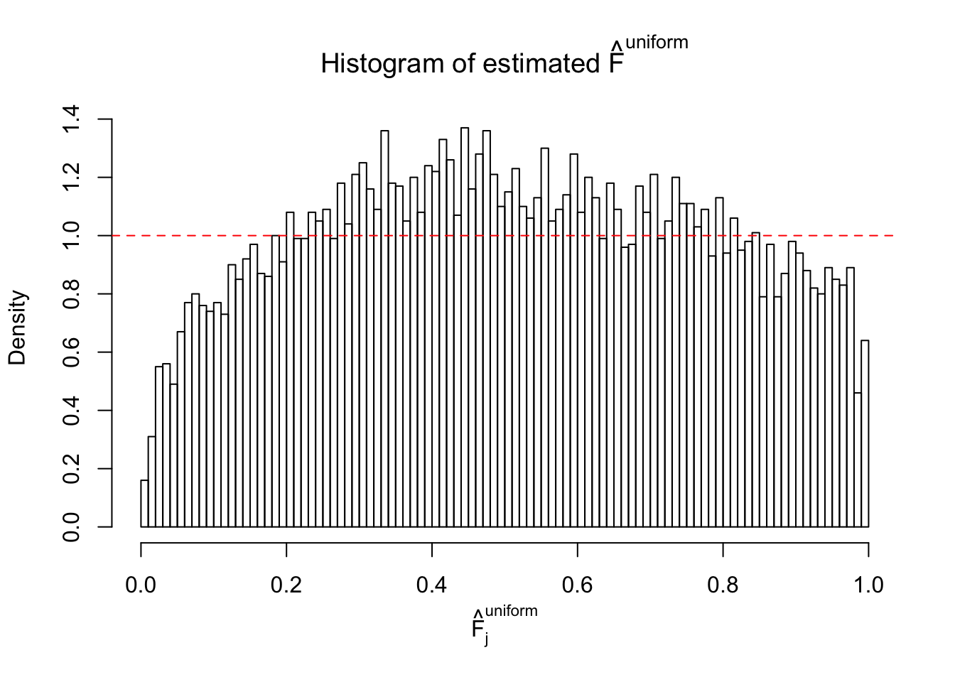
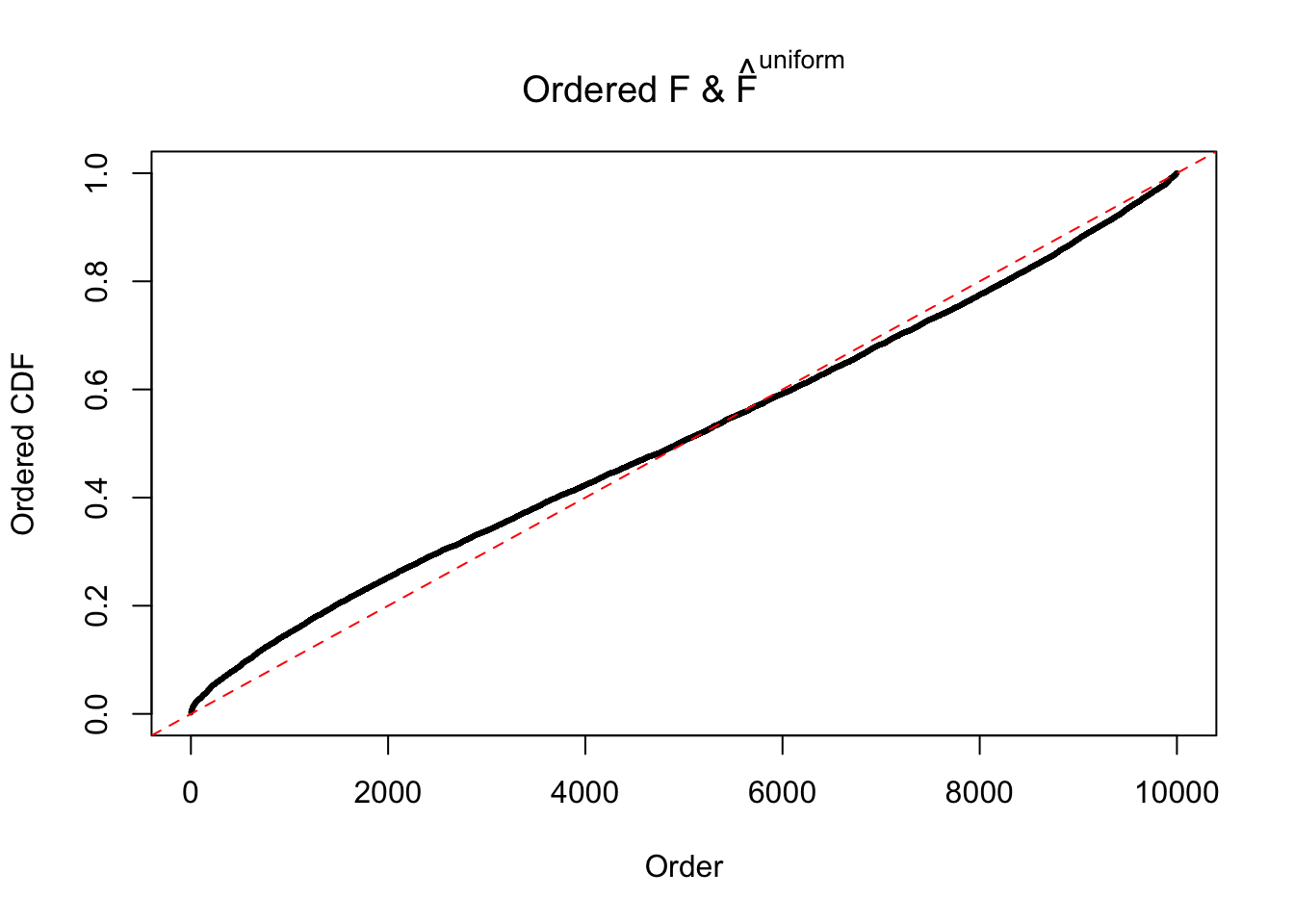
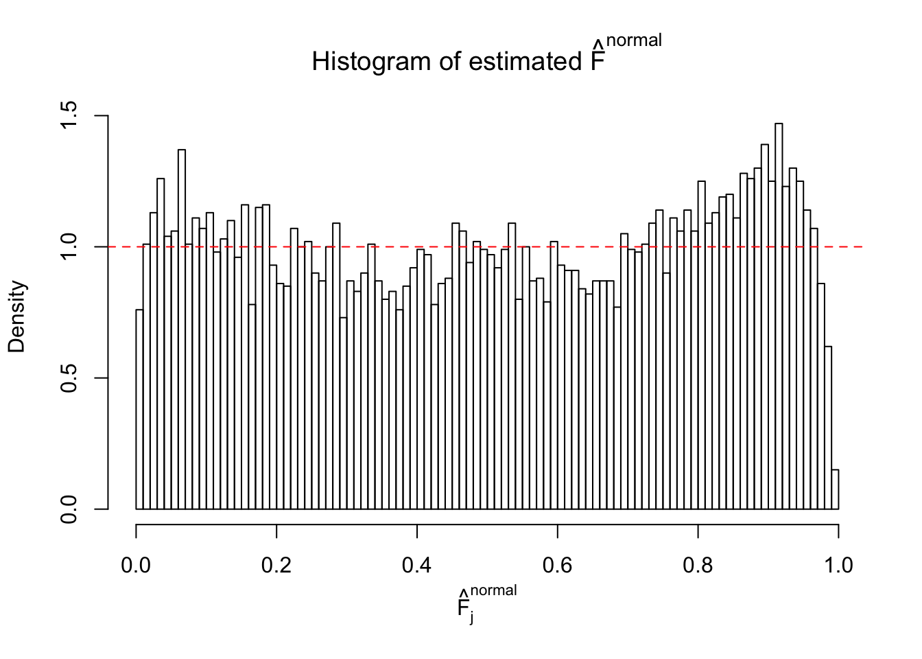
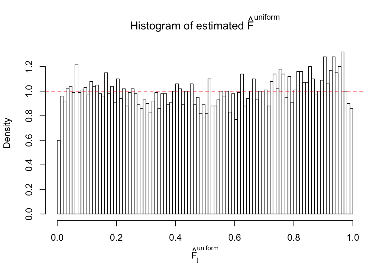
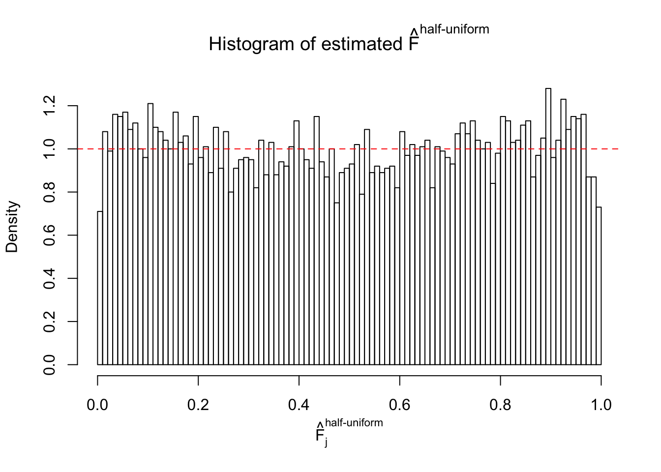
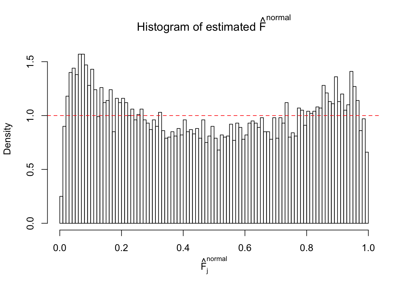
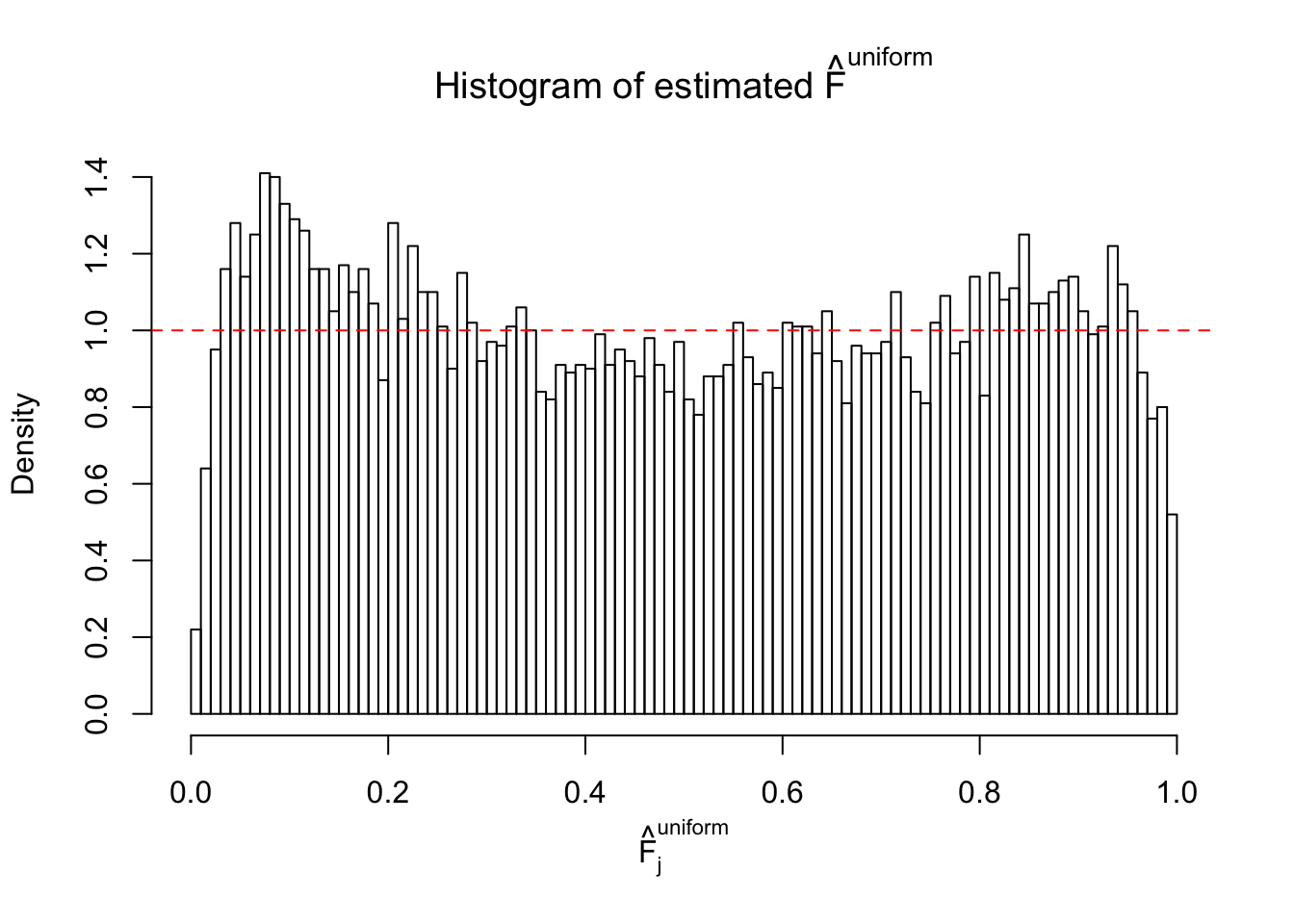
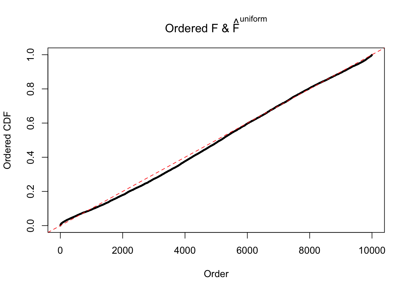
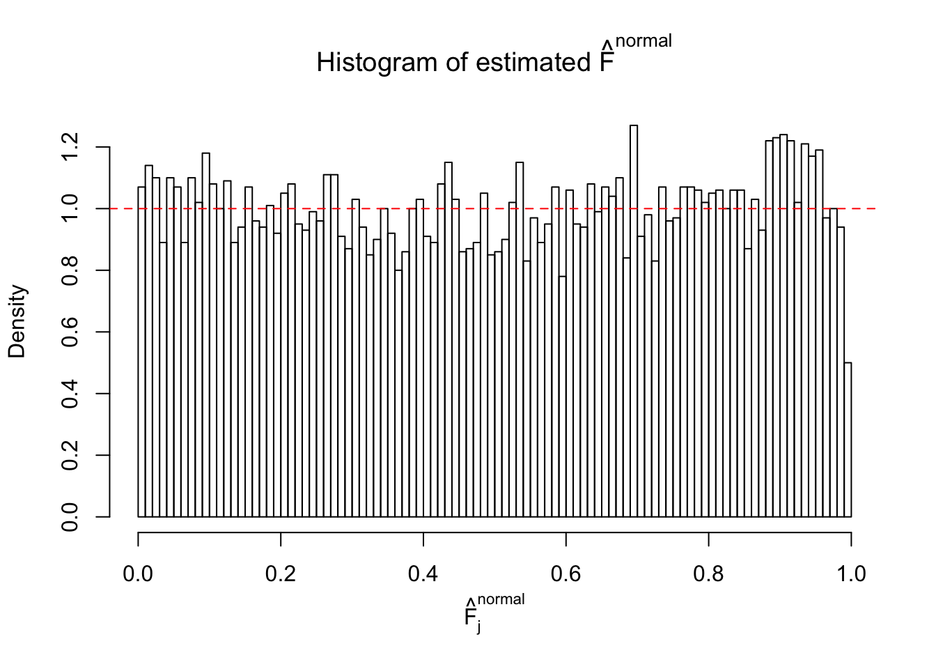
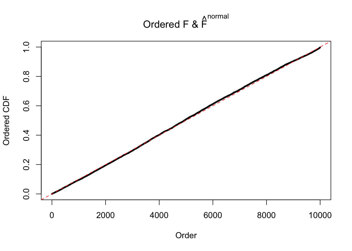
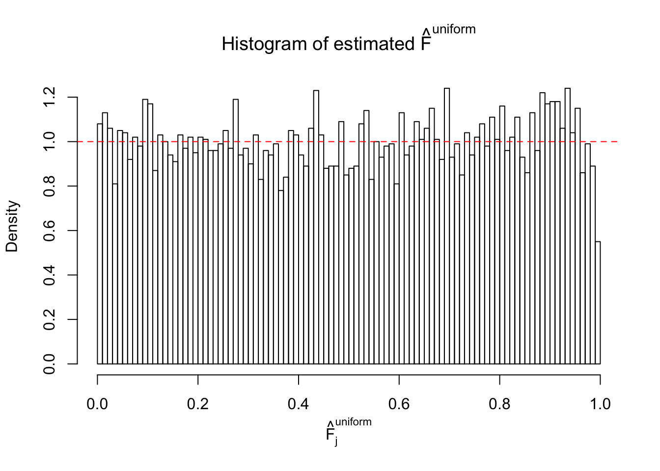
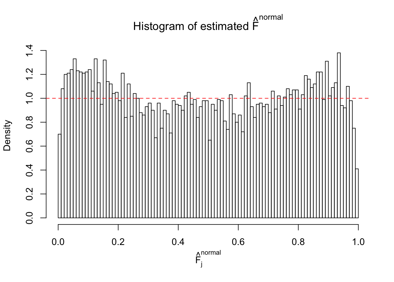
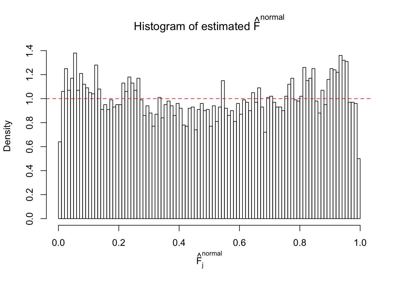
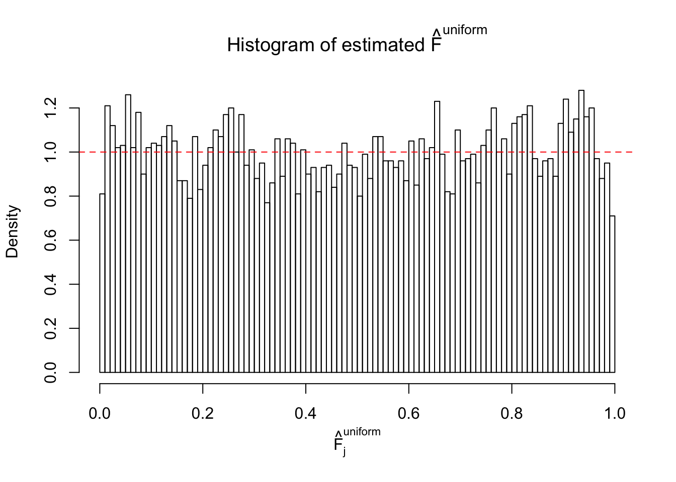
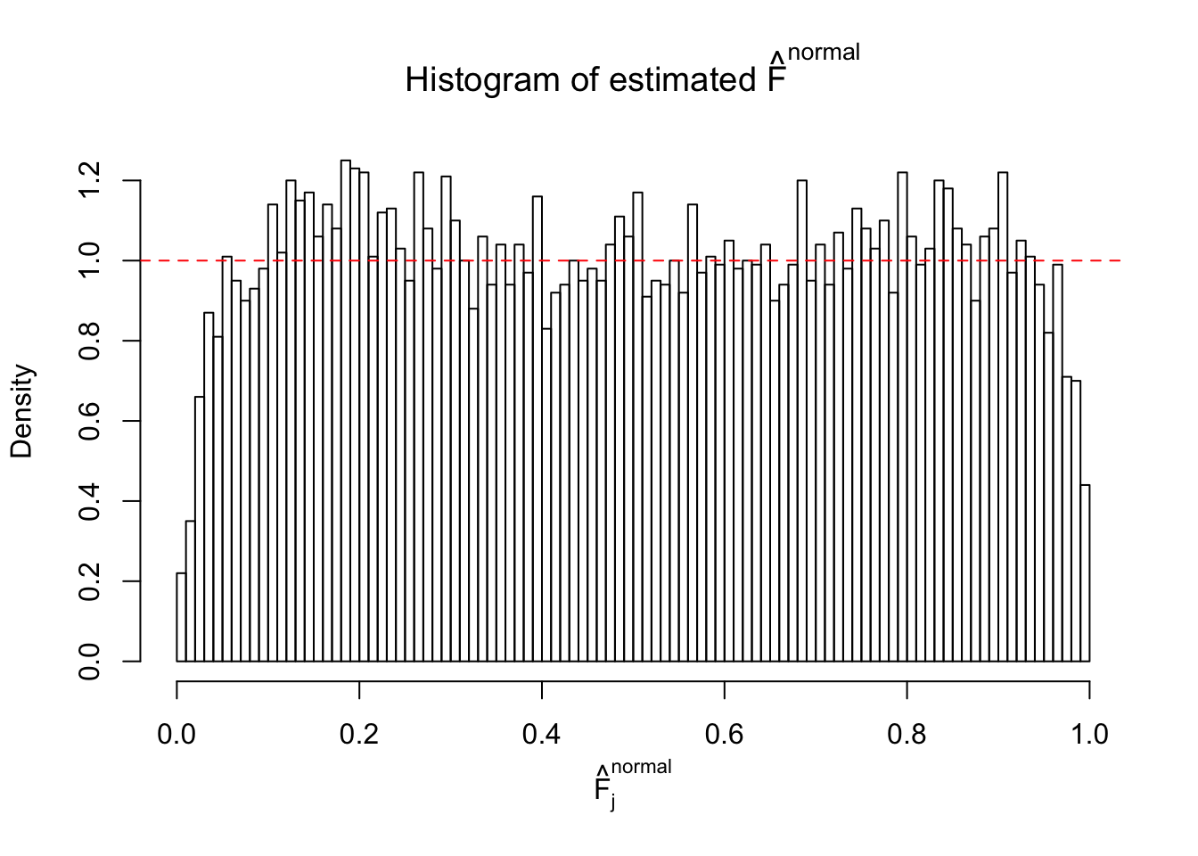
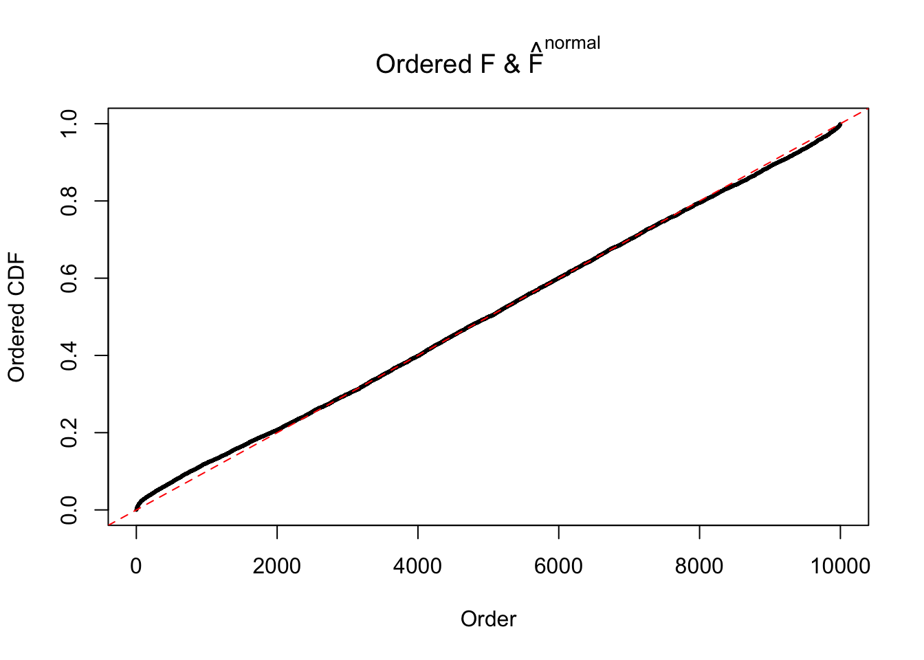
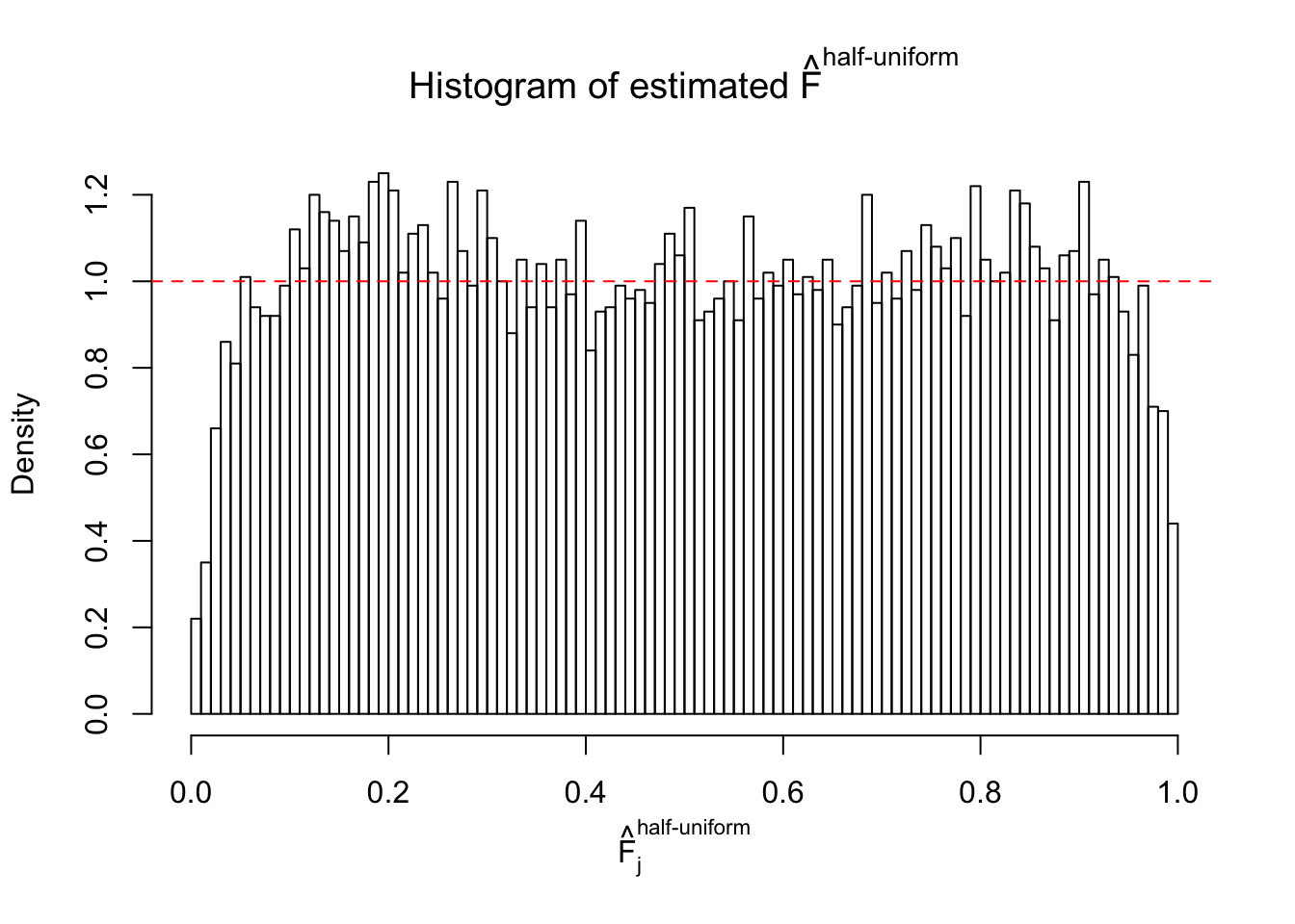
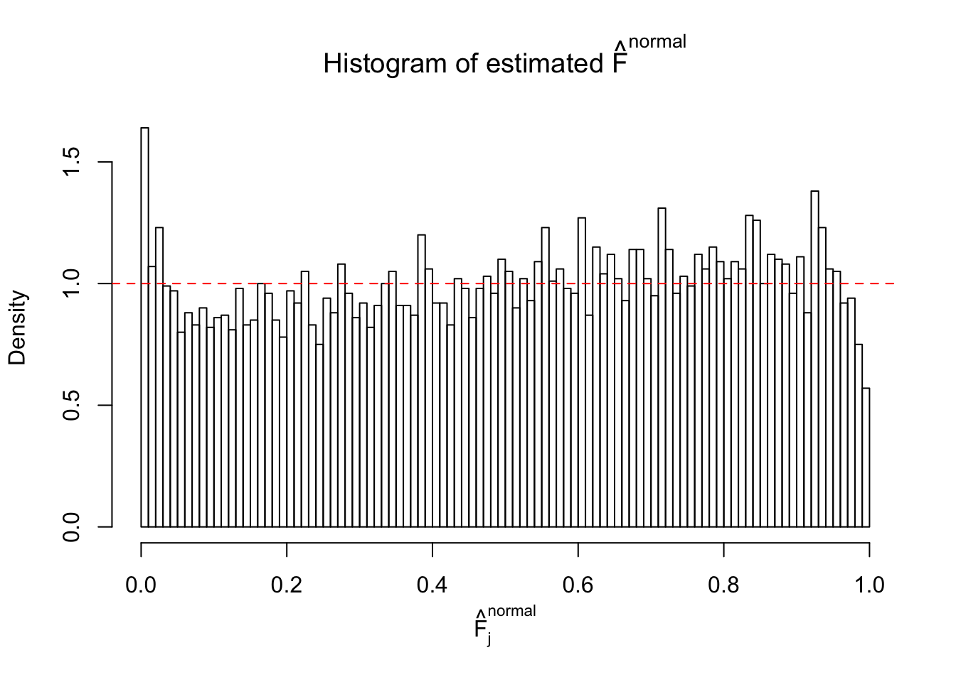
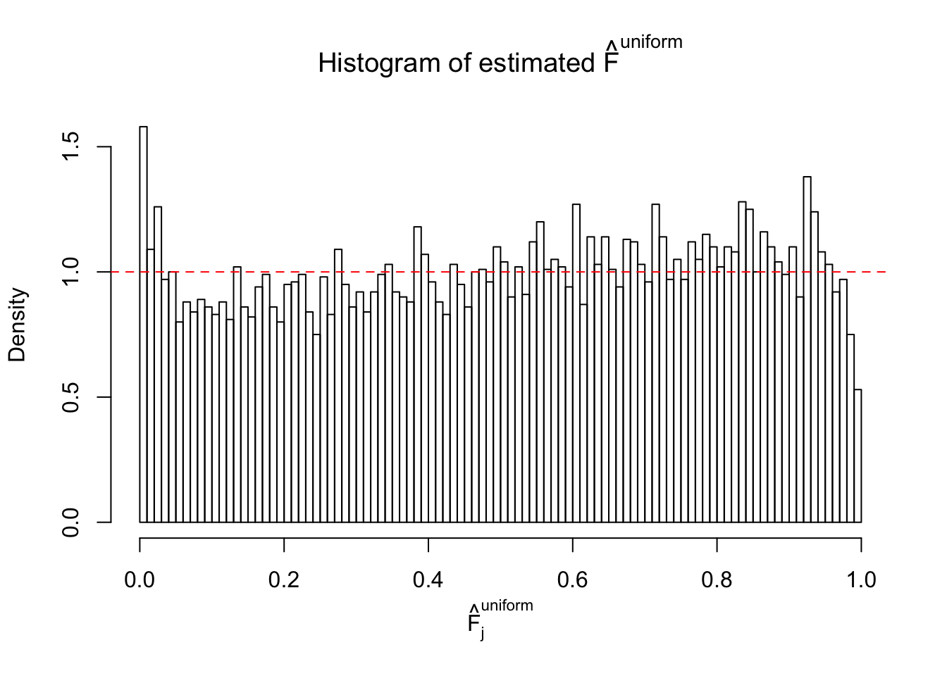
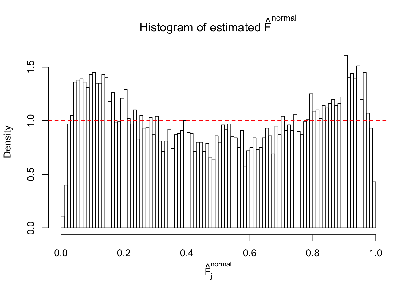
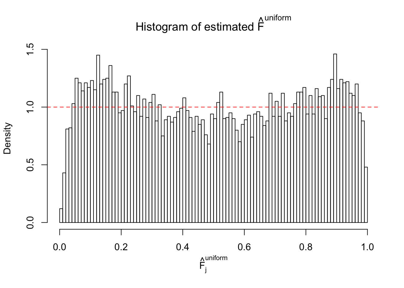
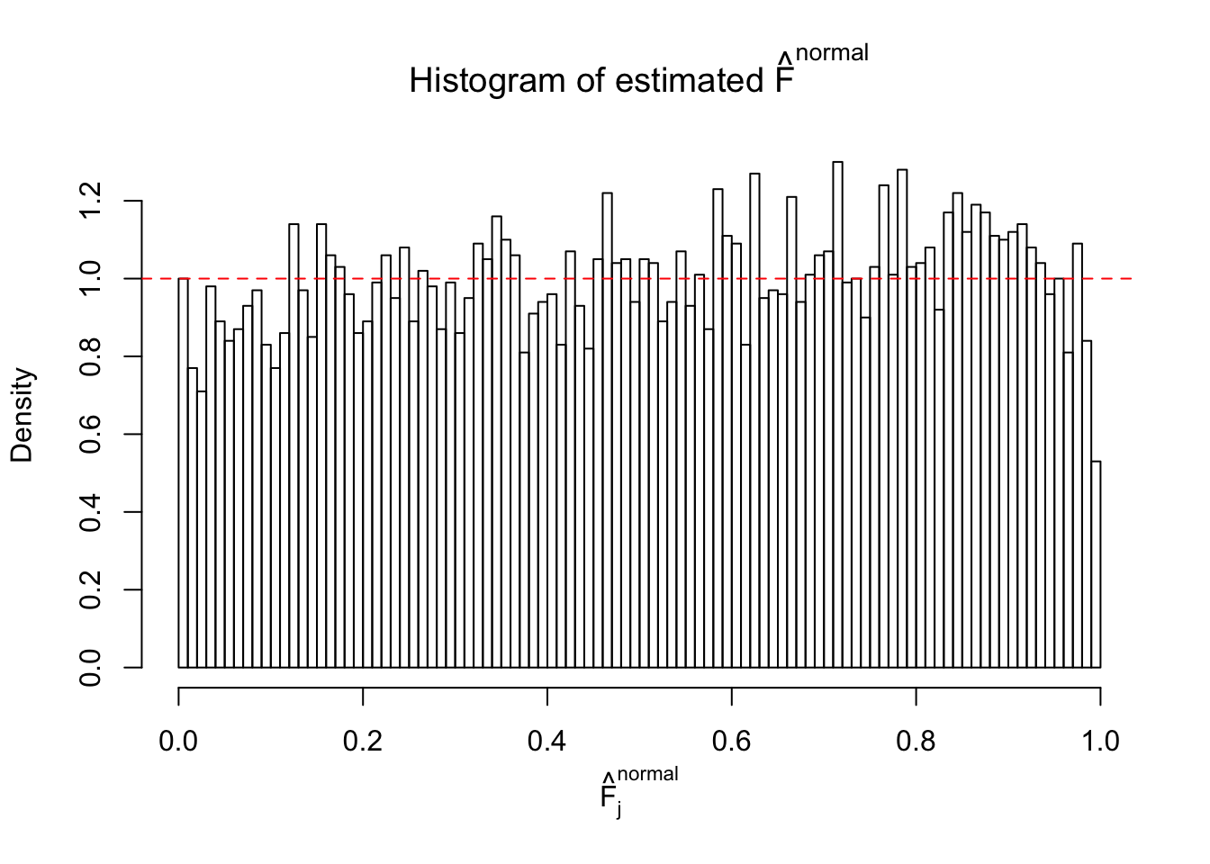
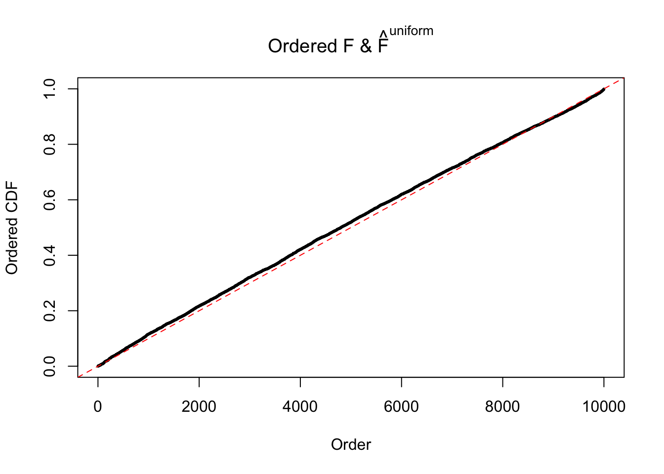
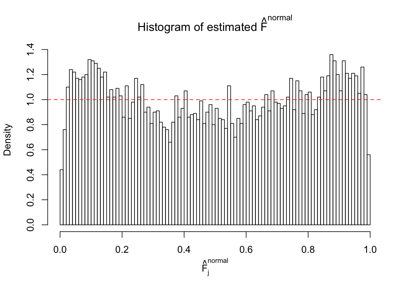
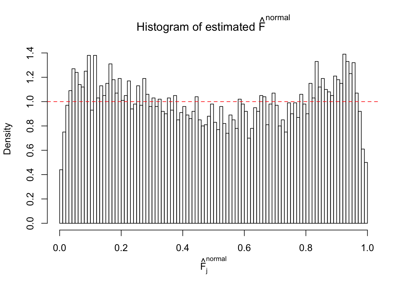
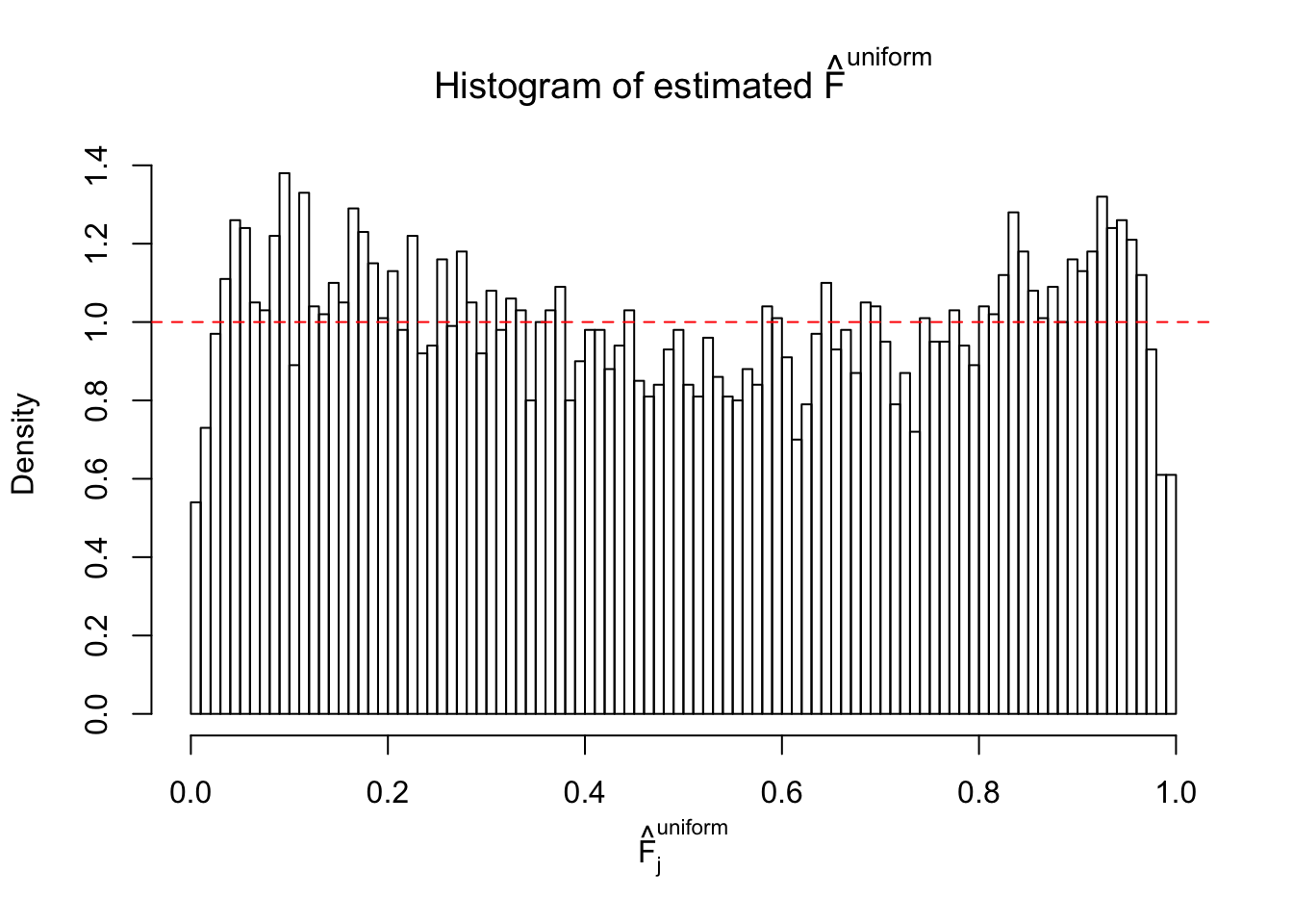
Diagnostic plots for ASH can be used to measure the goodness of fit of ASH. Breaking any of the assumptions behind ASH would make its fit less well, as shown in the non-uniformness of \(\left\{\hat F_j\right\}\), among which some cases have been discussed.
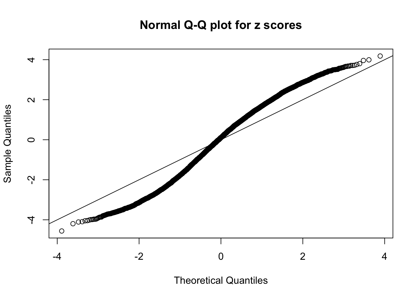
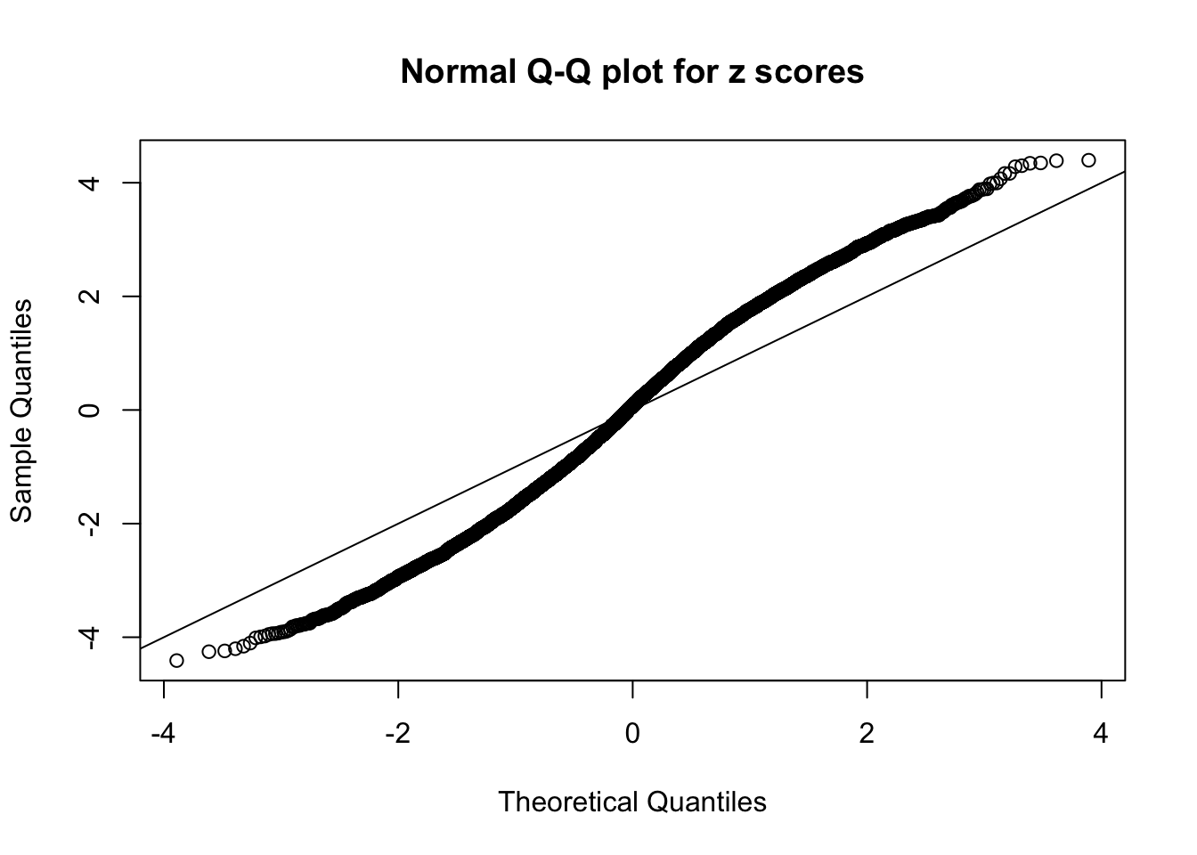
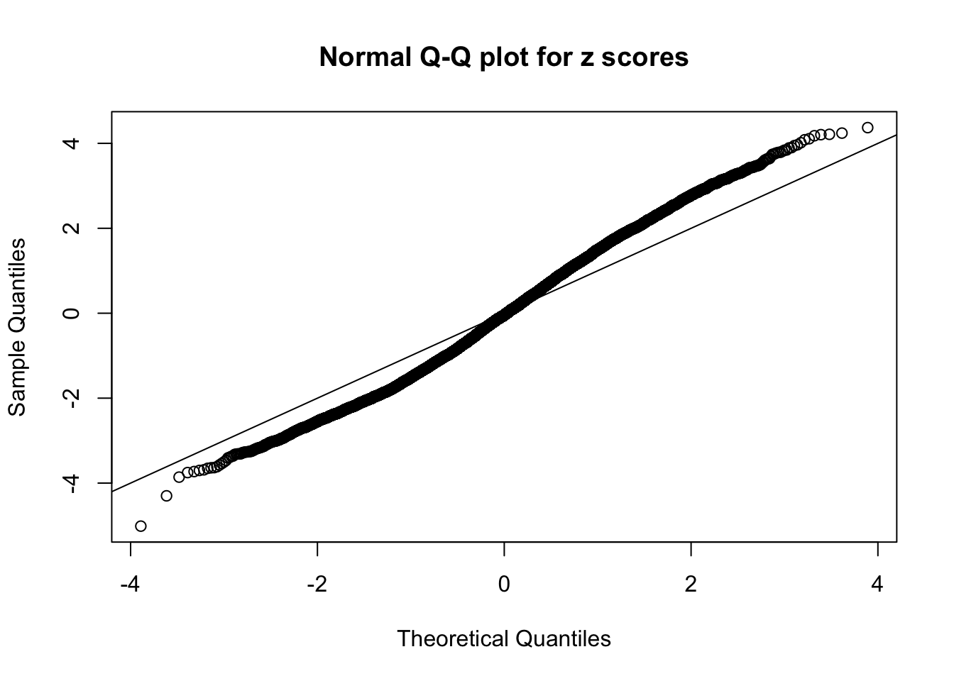
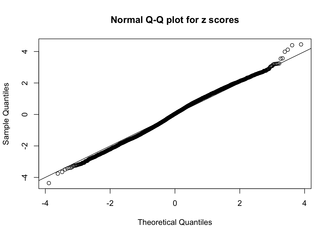
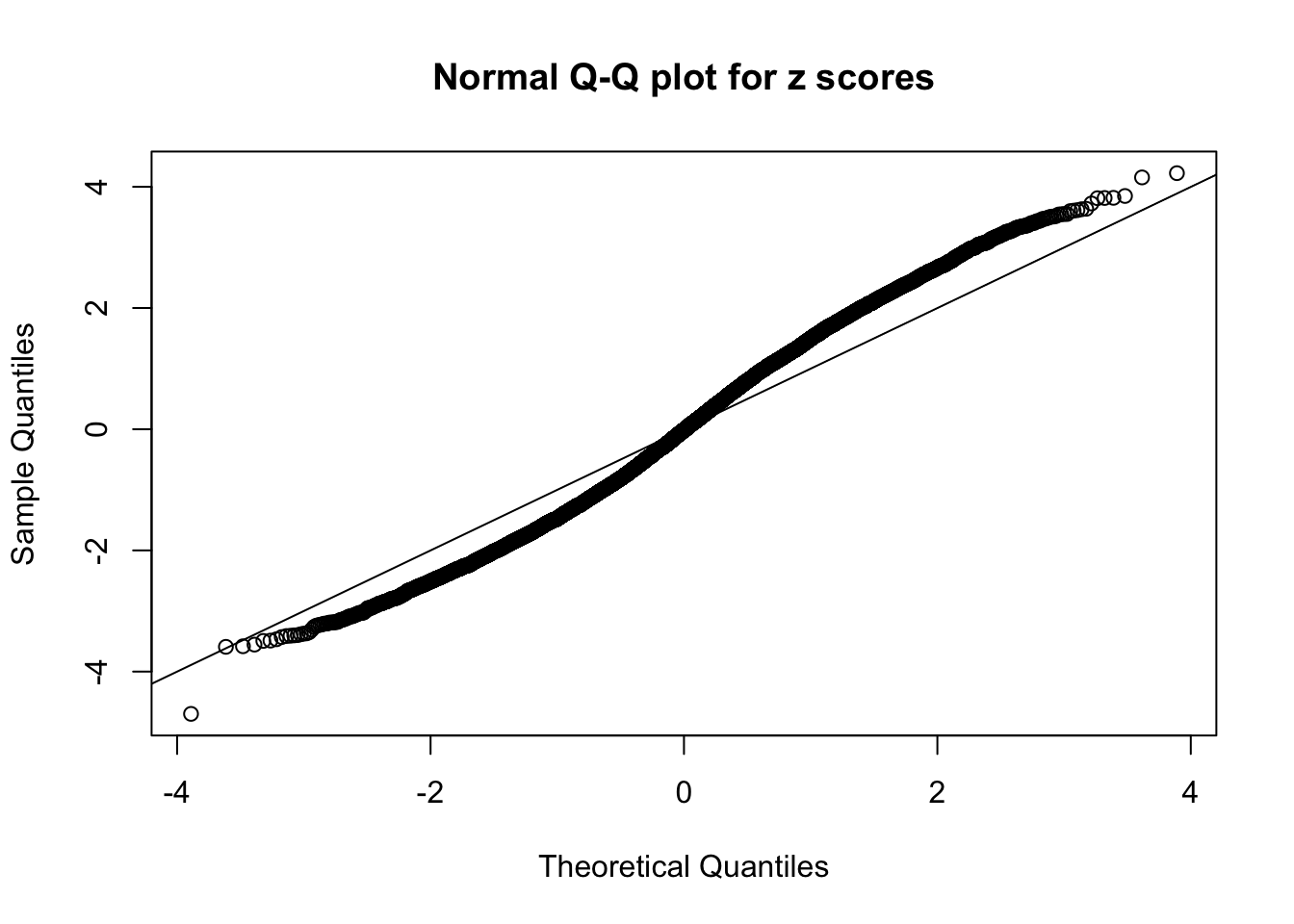
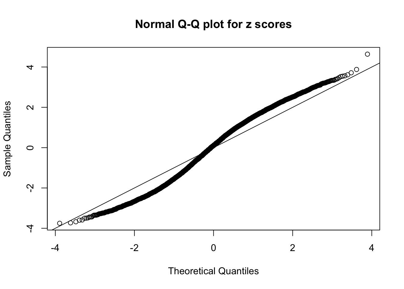
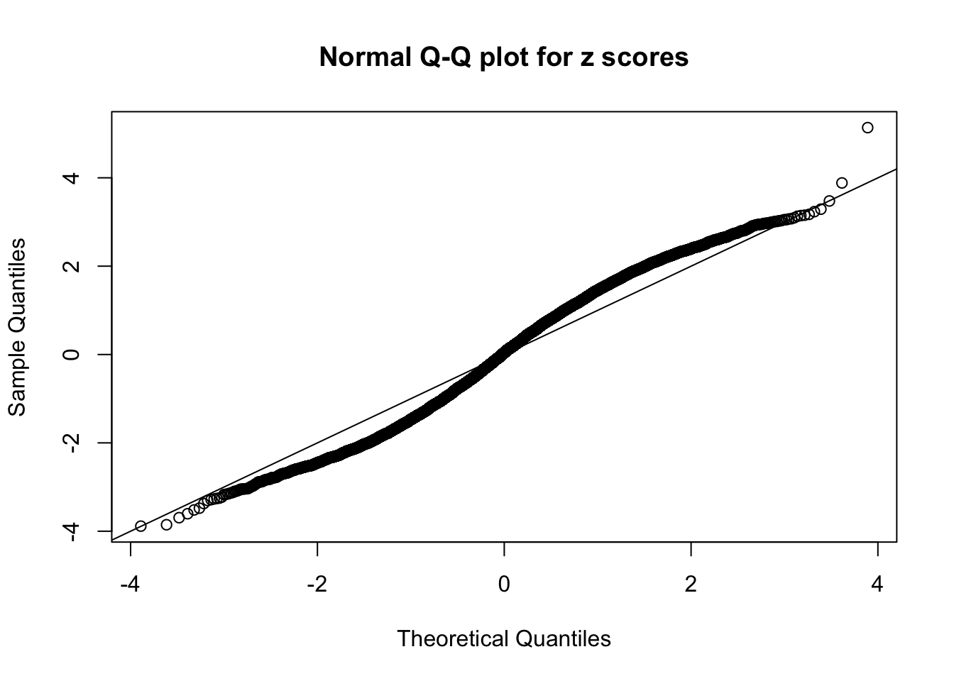
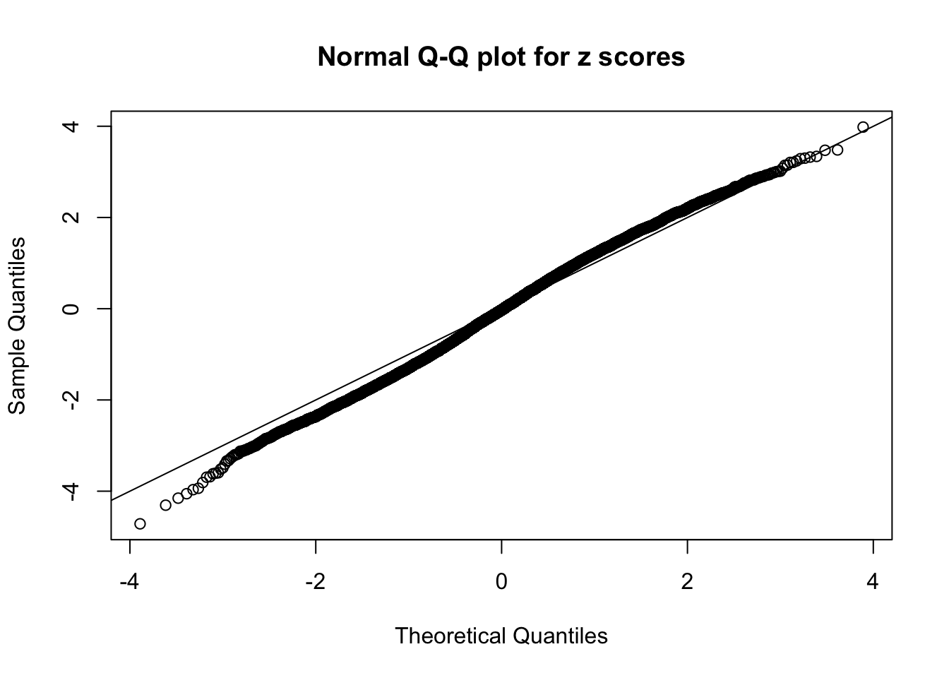
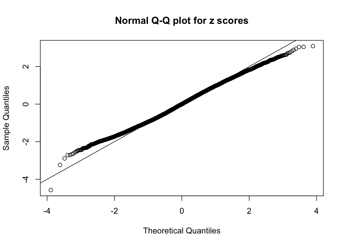
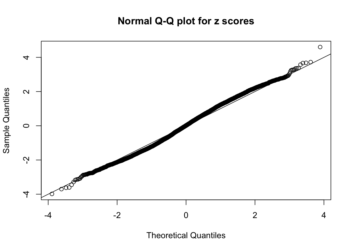
A special case closely related to this project is about correlation. The presence of correlation could affects the accuracy of estimating \(g\), as shown before. Moreover, the correlation will inflate the empirical distribution of the correlated noise, making it less regular, thus less able to be captured by the mixture of normals or uniforms as in ASH.
Dignostic plots for all BH-hostile data sets
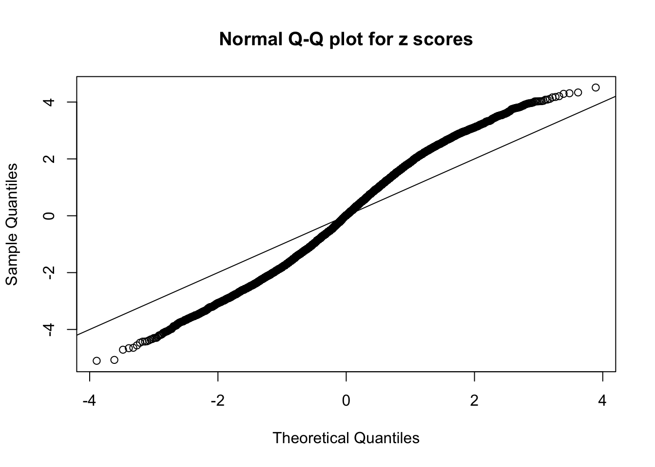
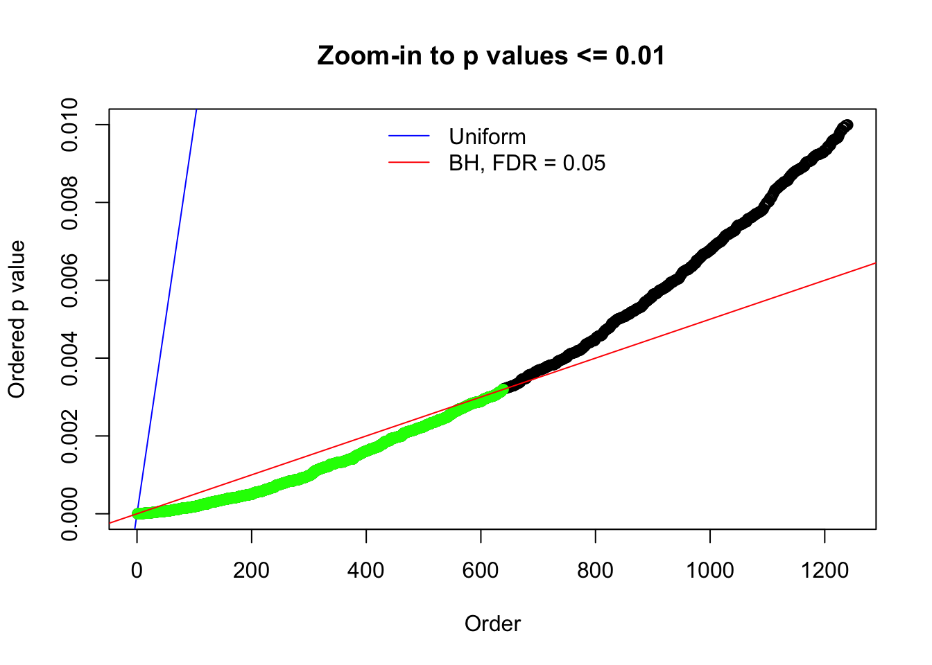
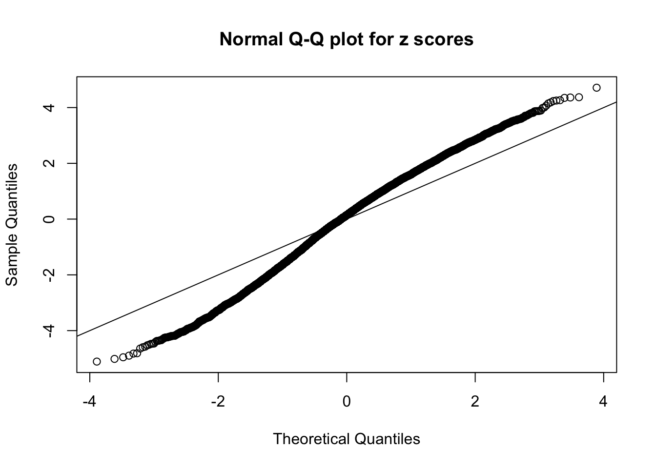
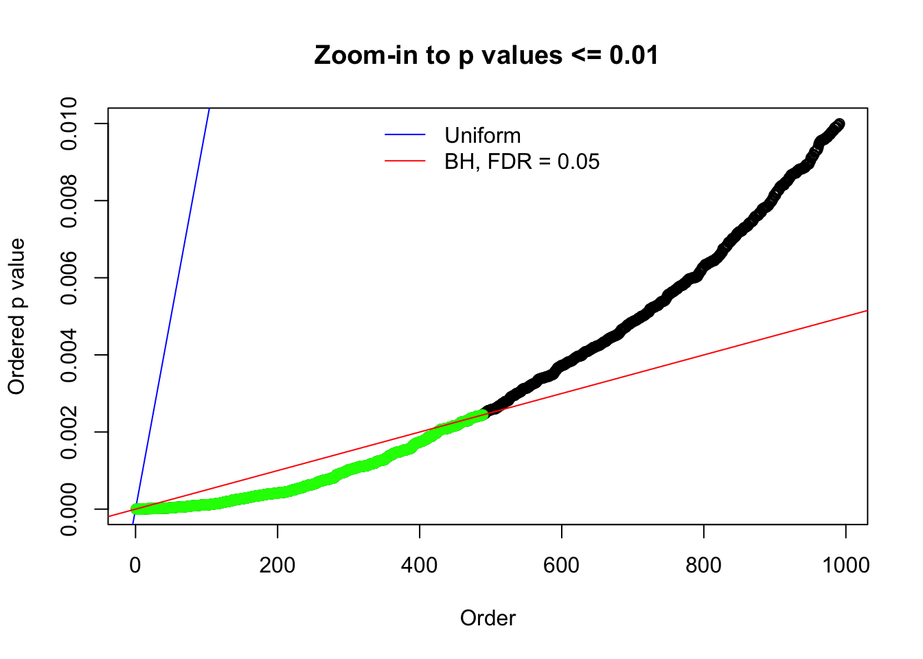
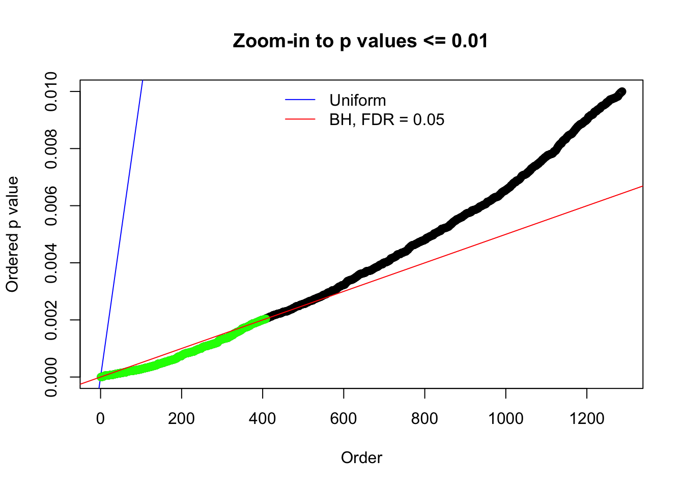
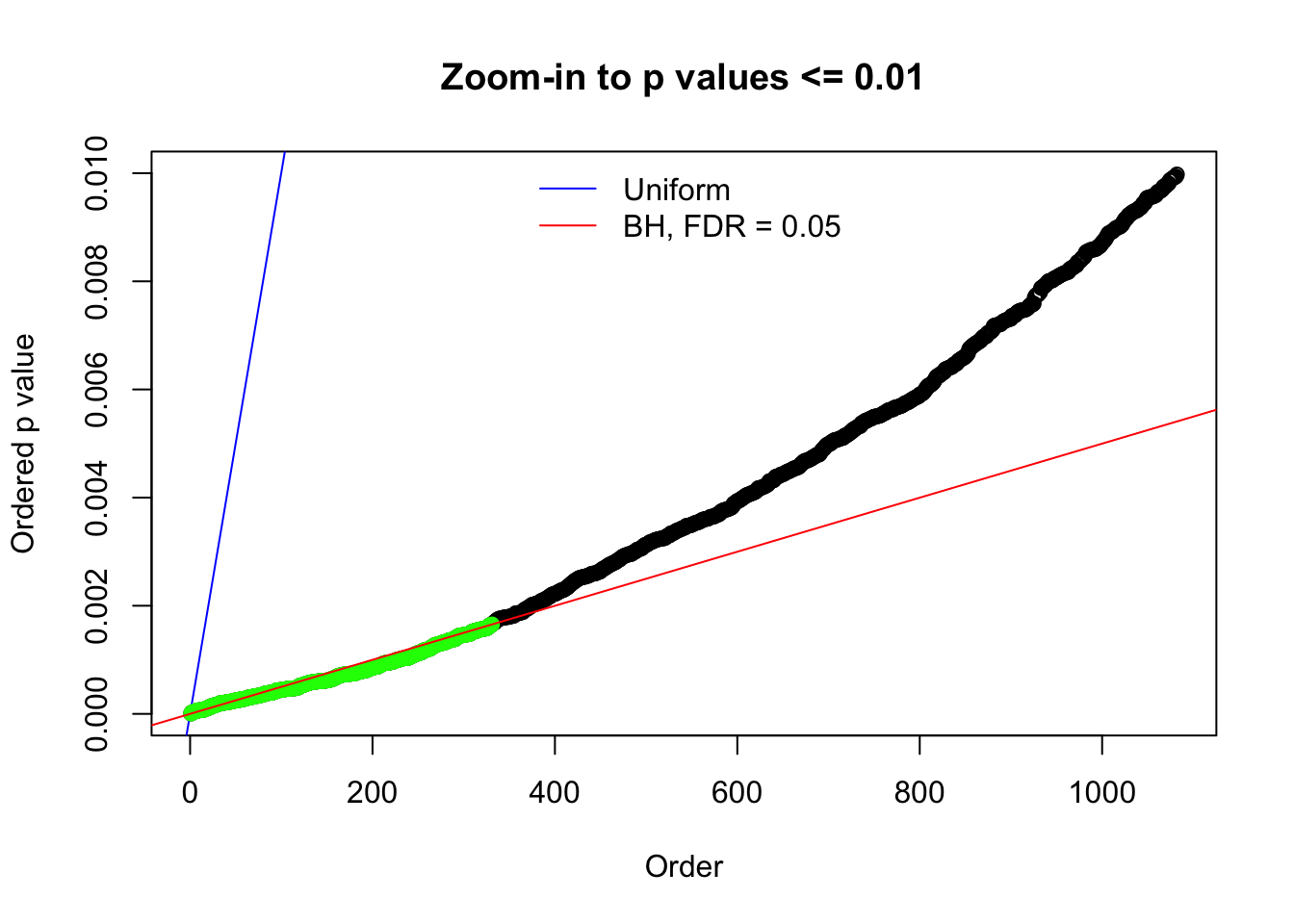
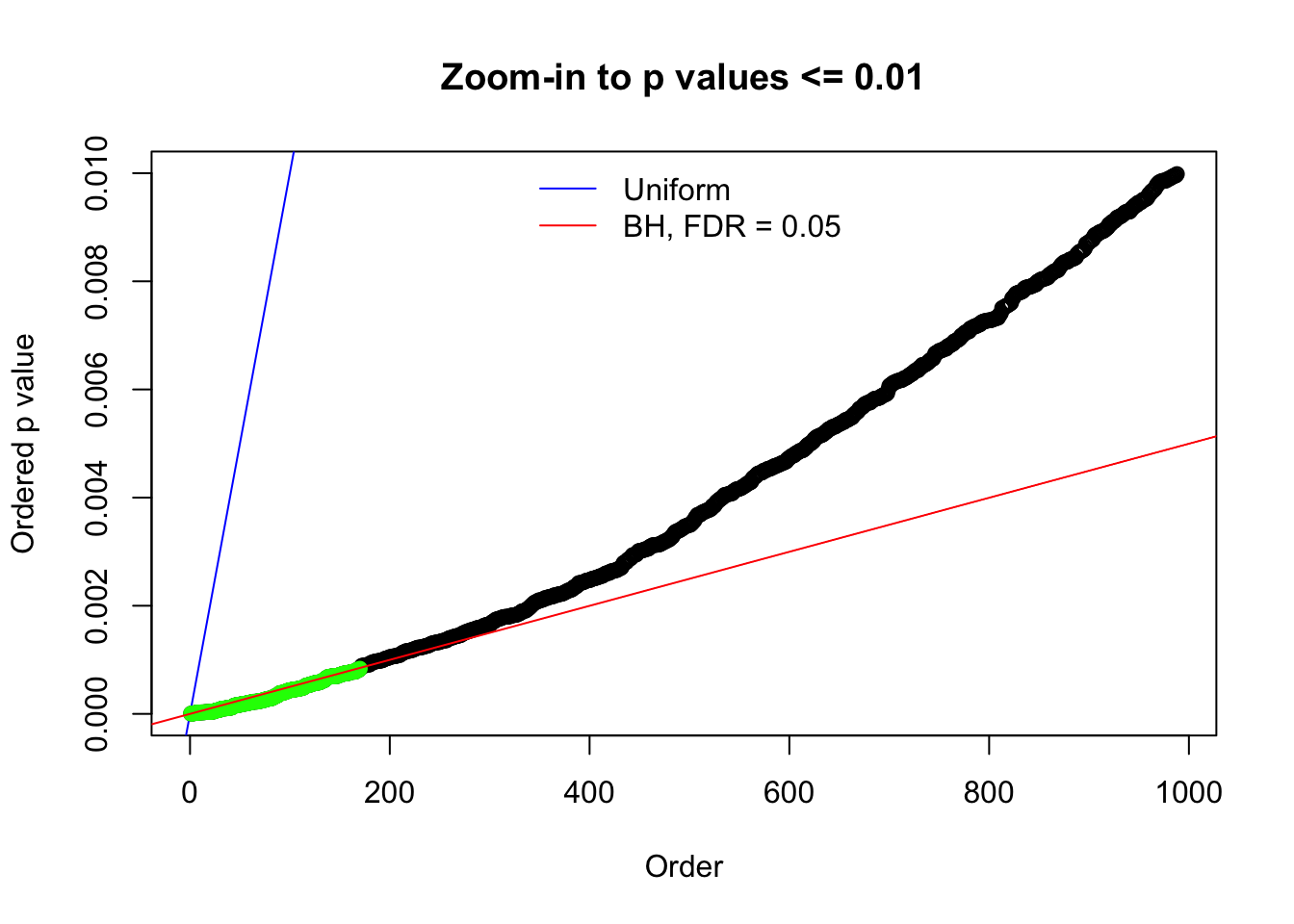
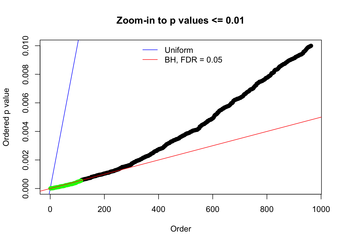
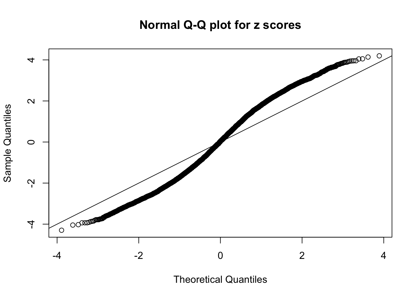
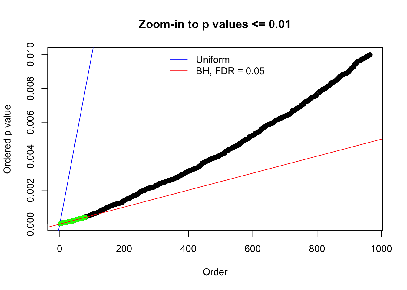
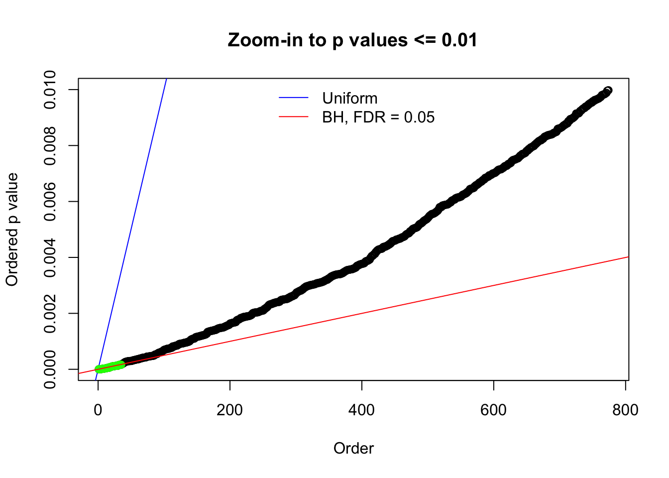
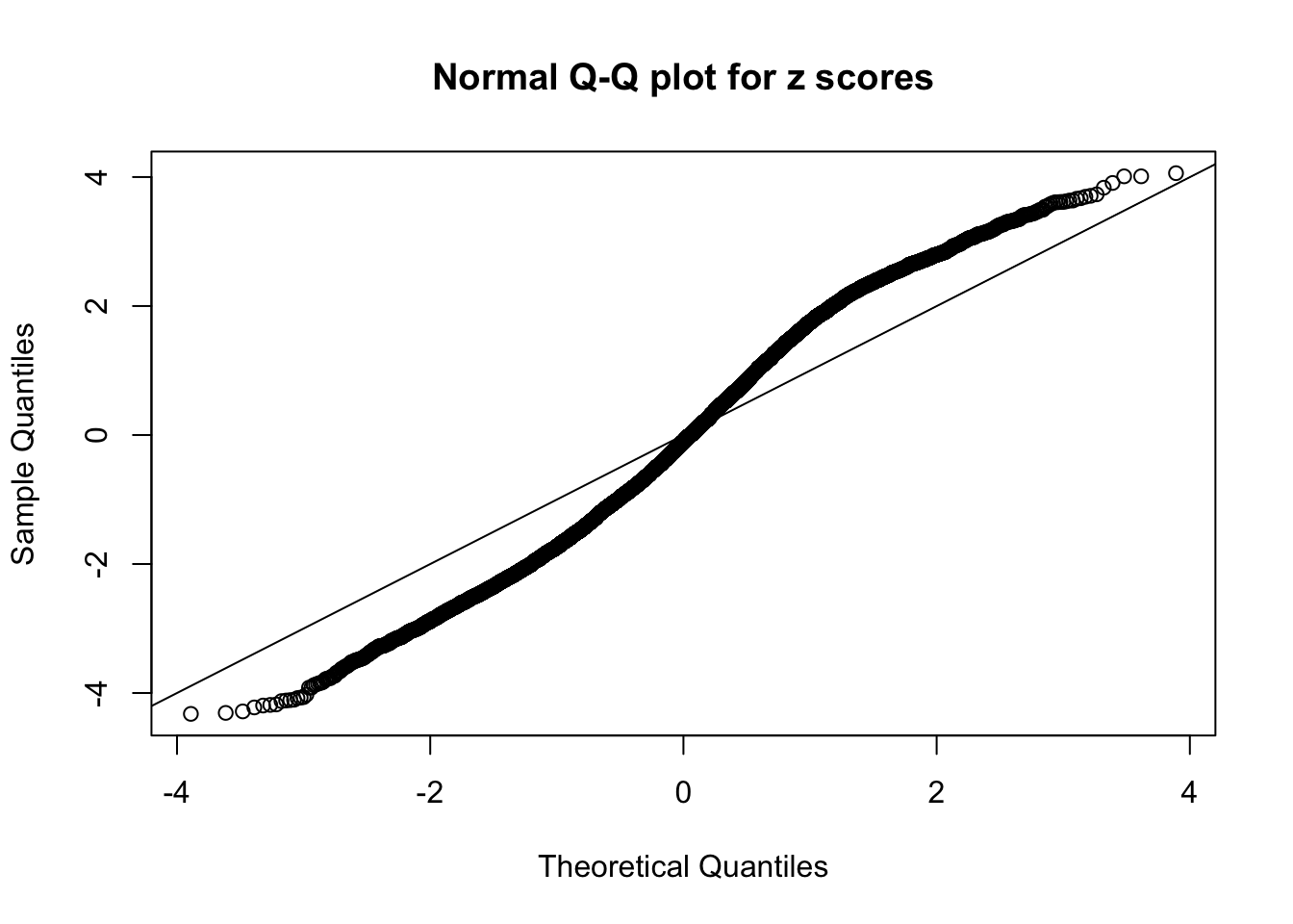
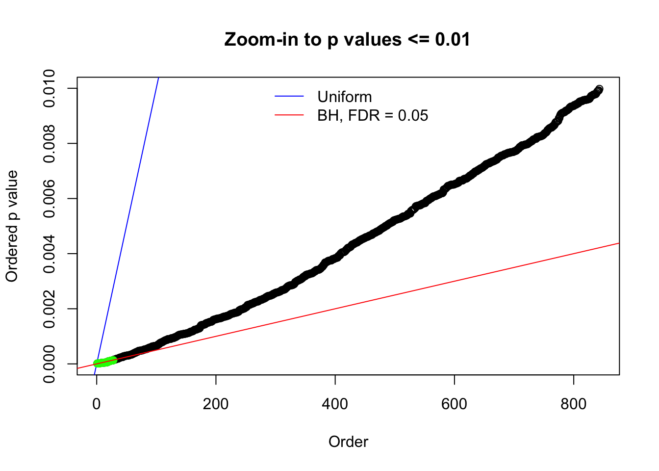
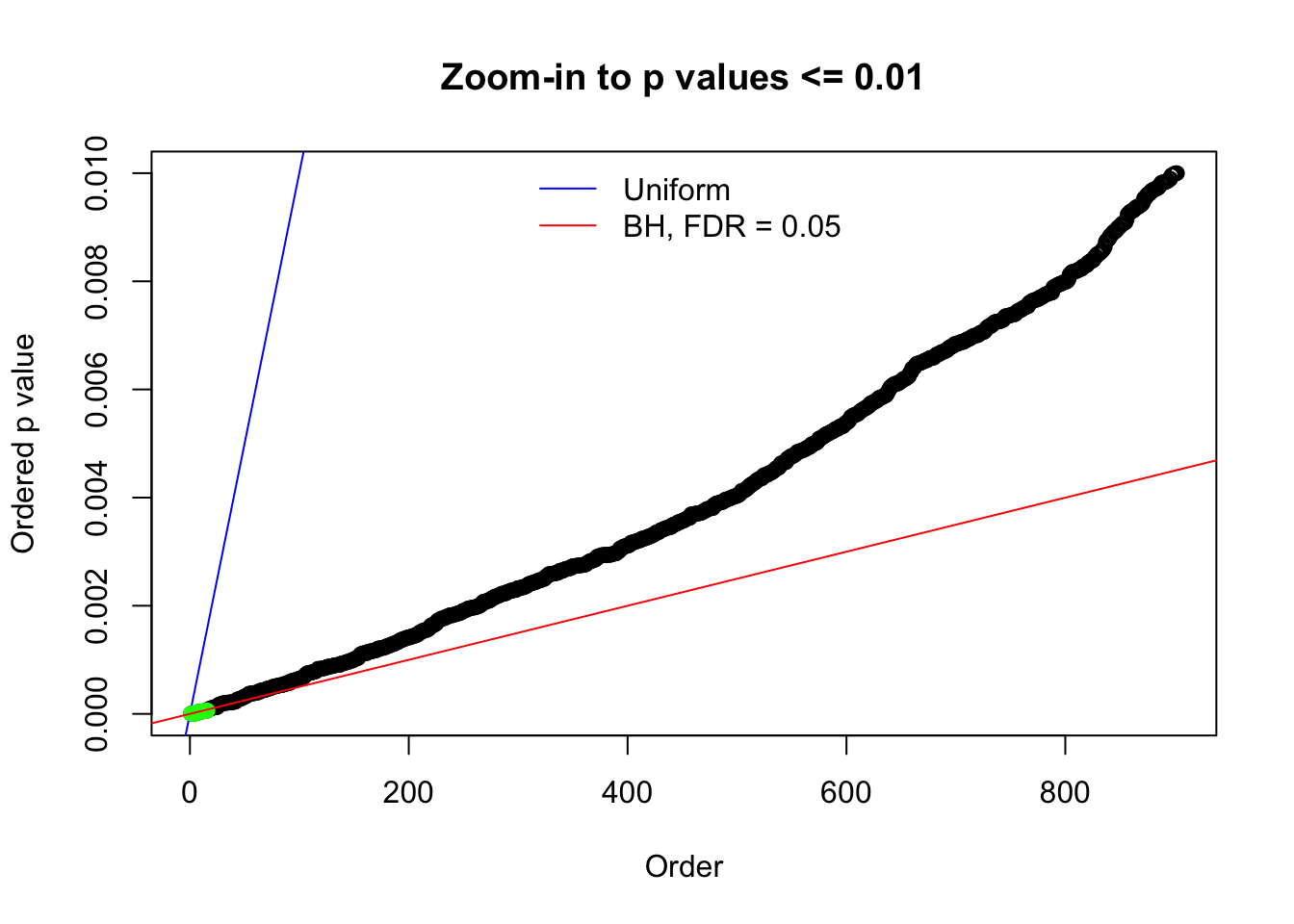
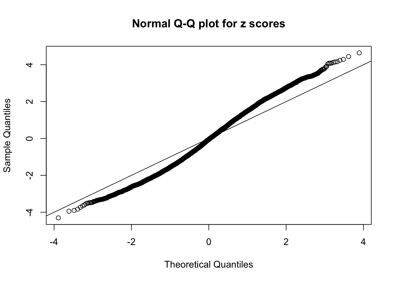
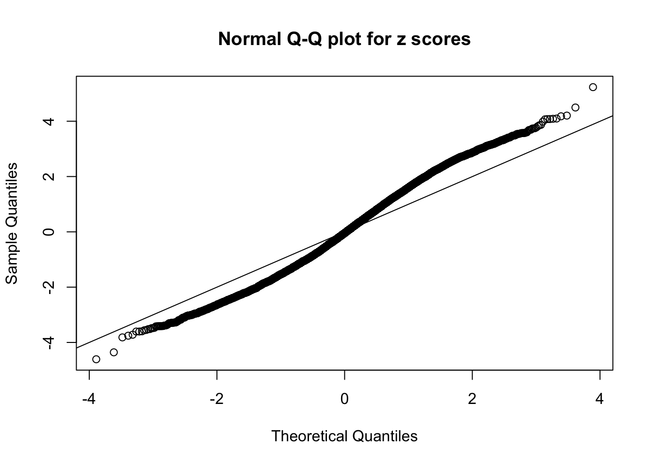
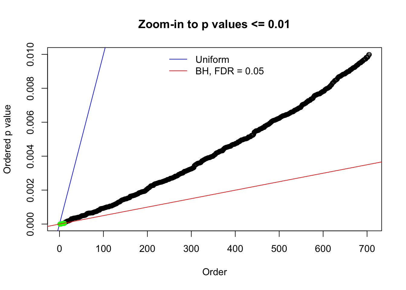
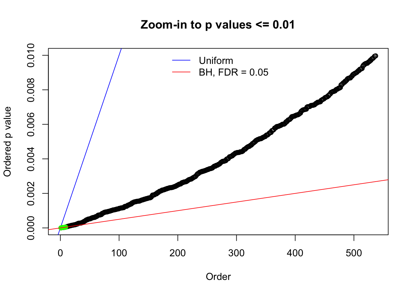
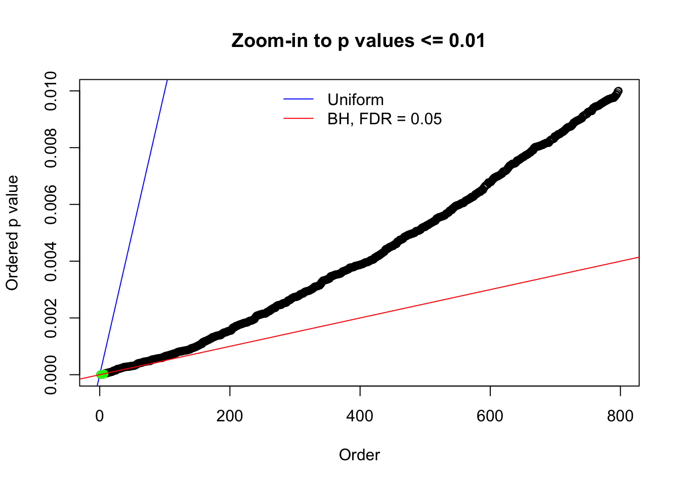
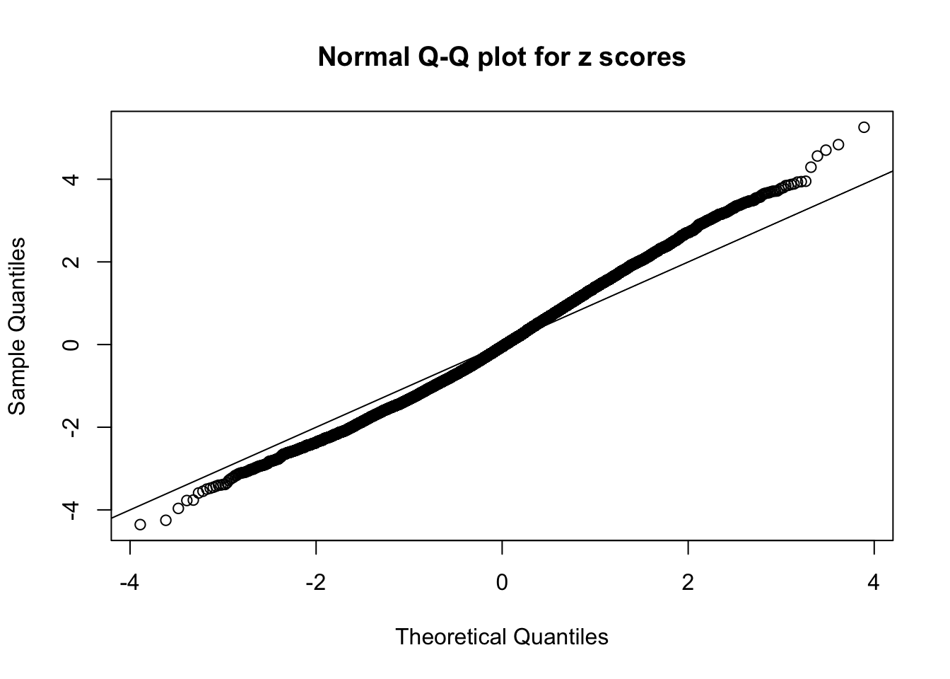
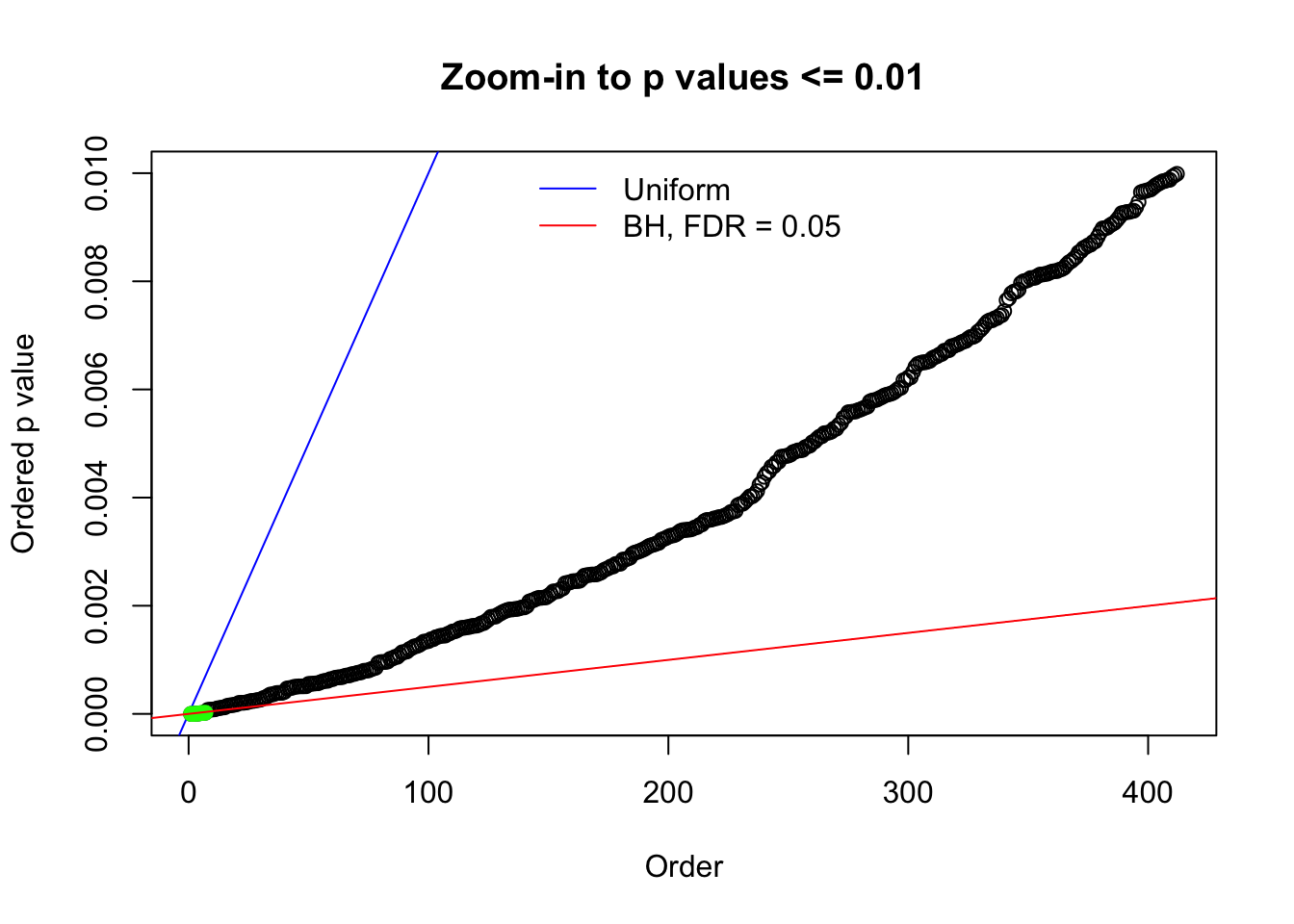
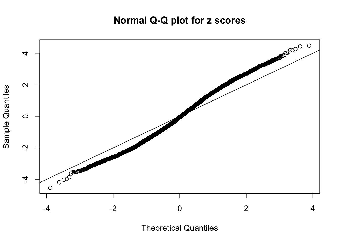
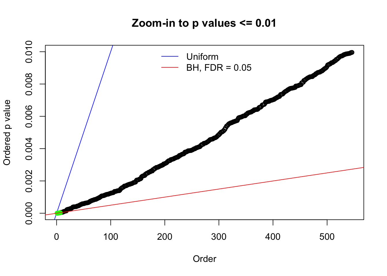
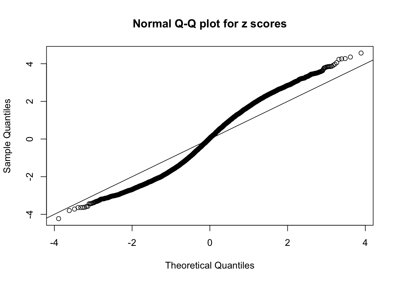
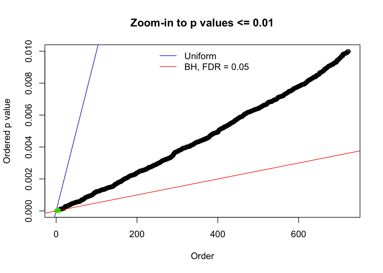
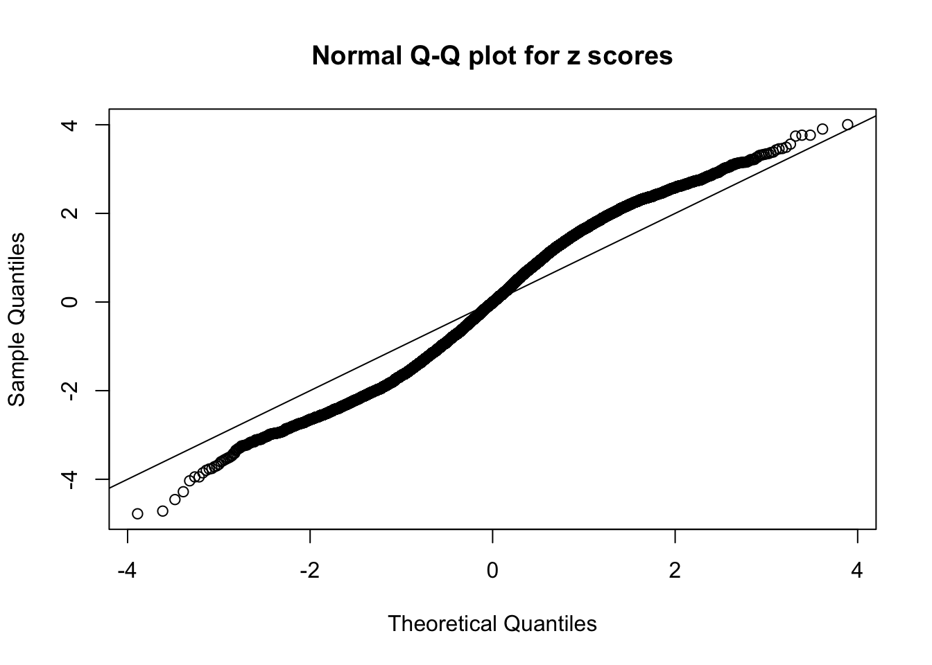
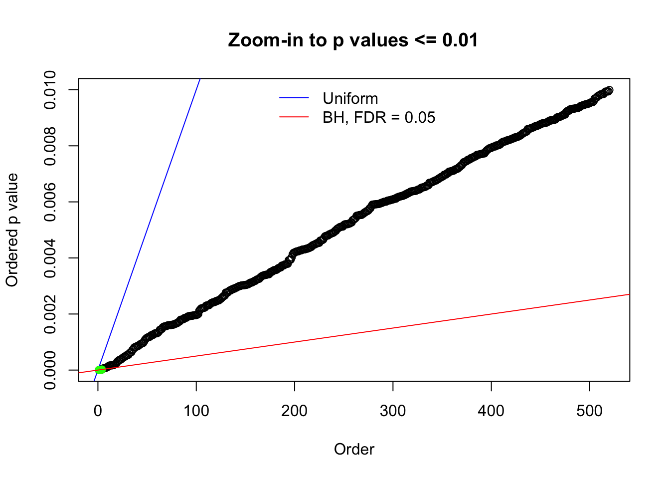
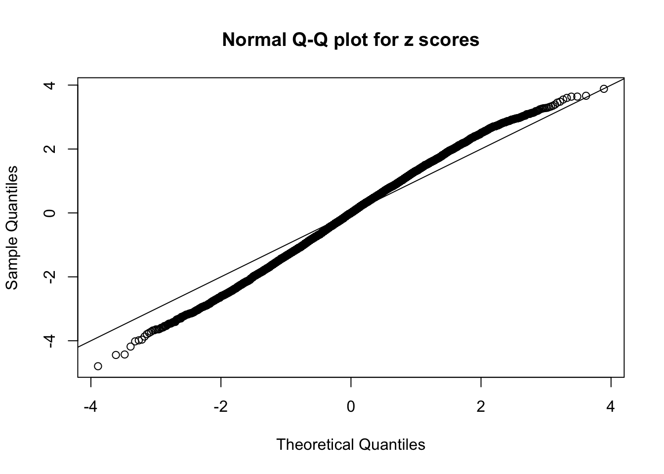
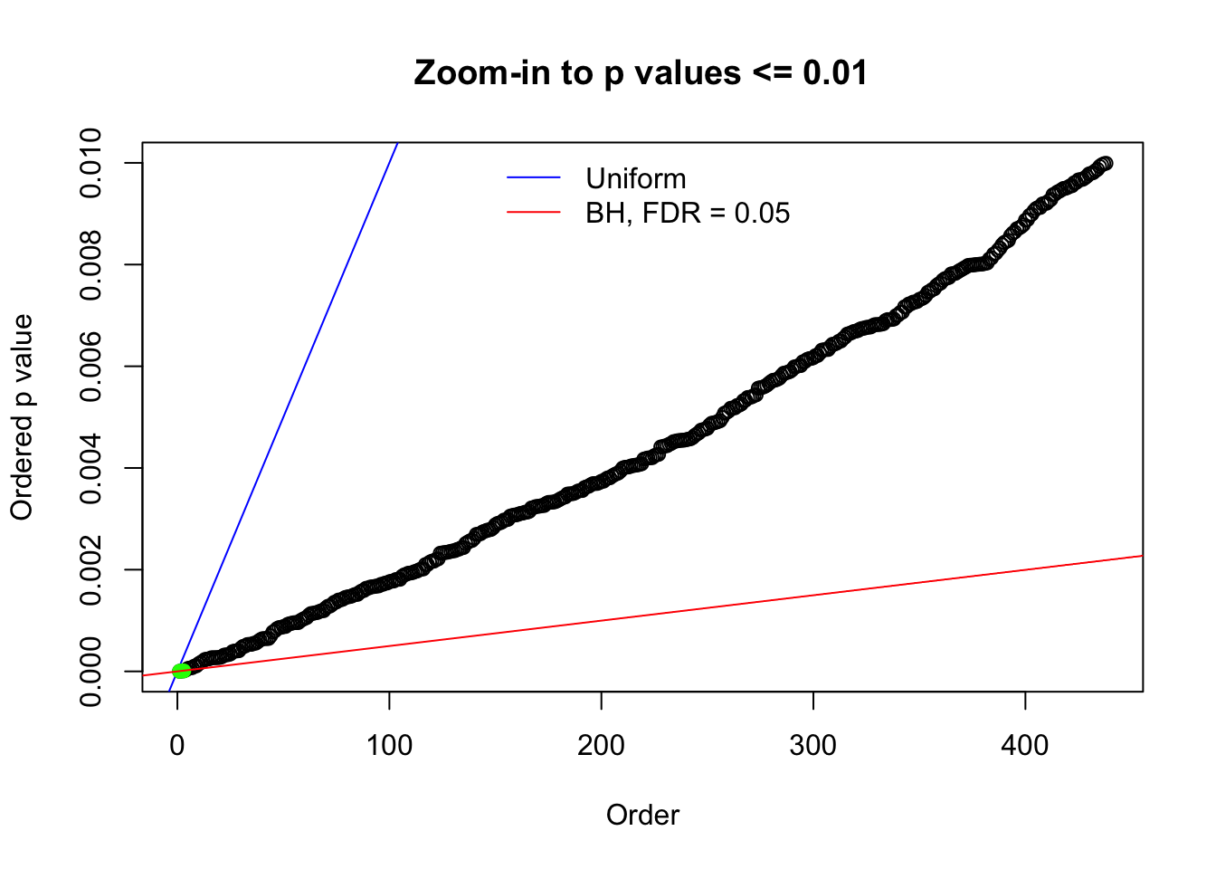
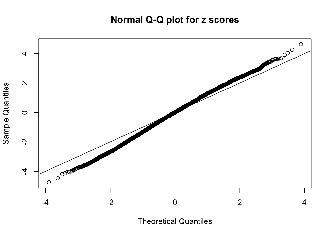
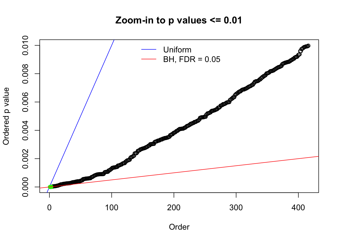
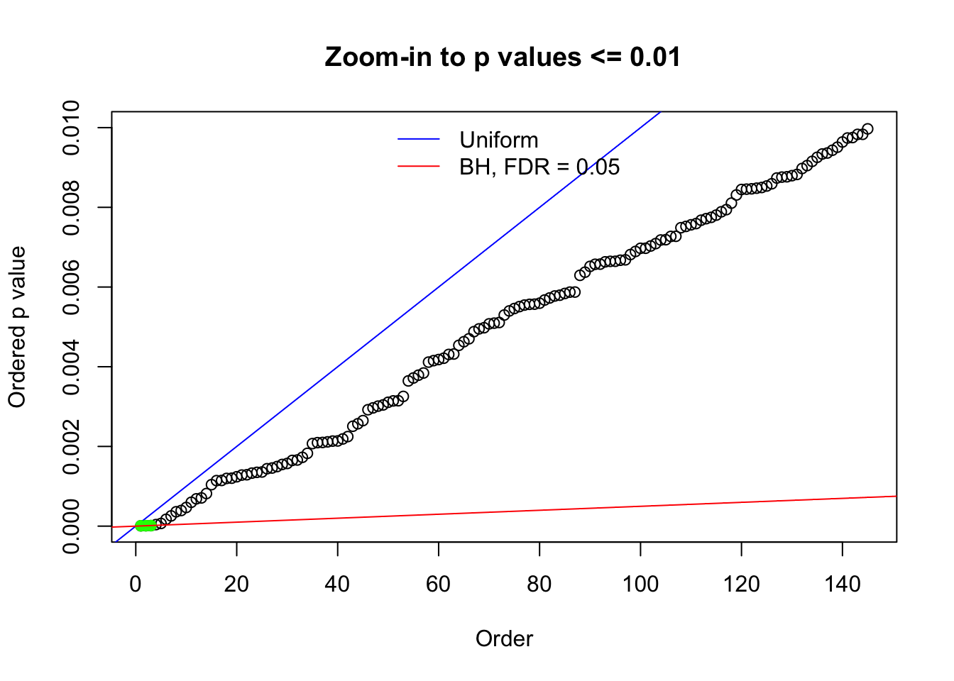
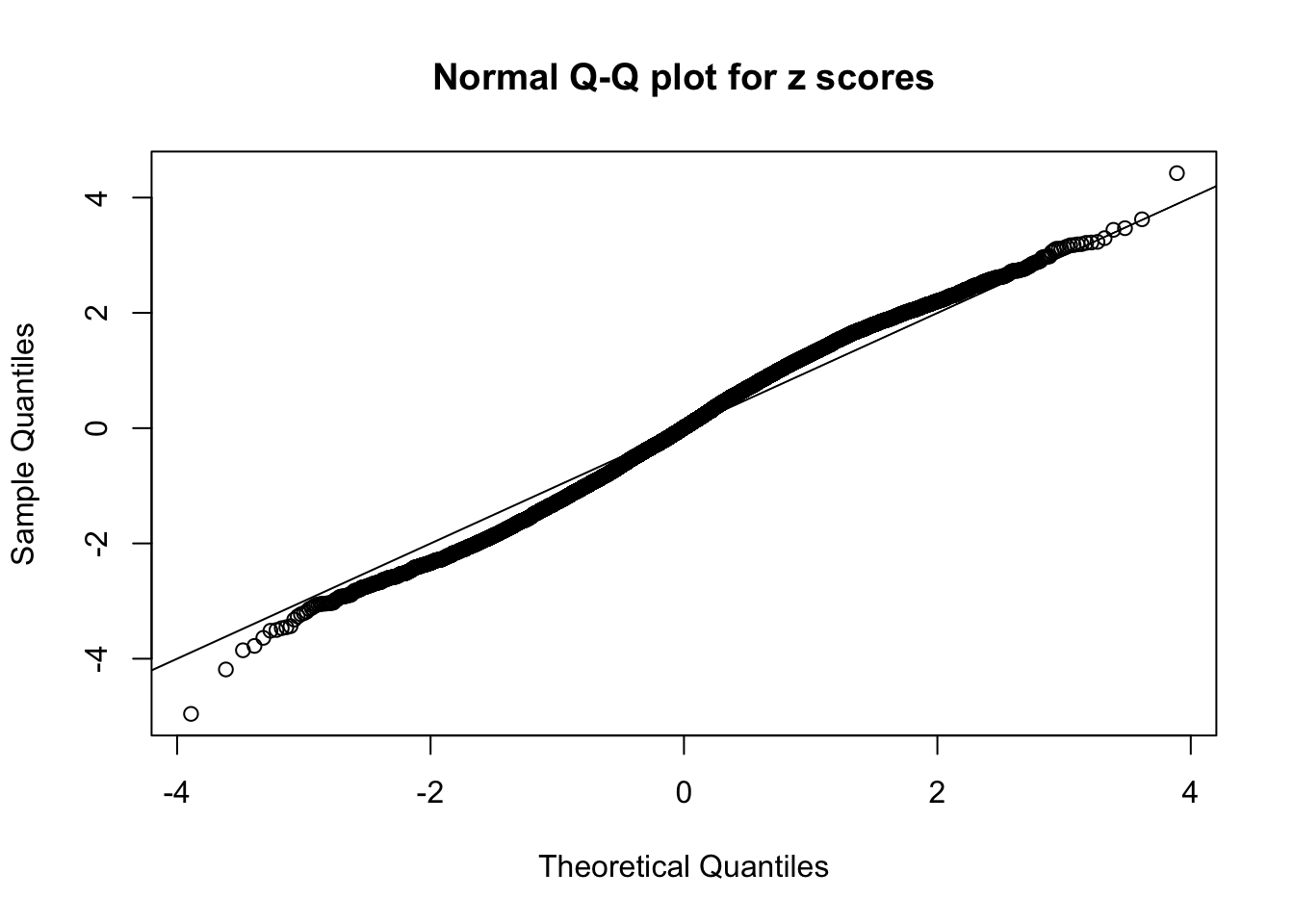
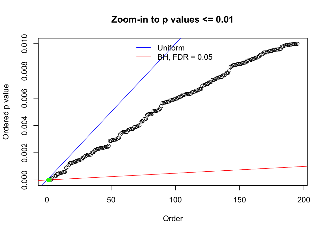
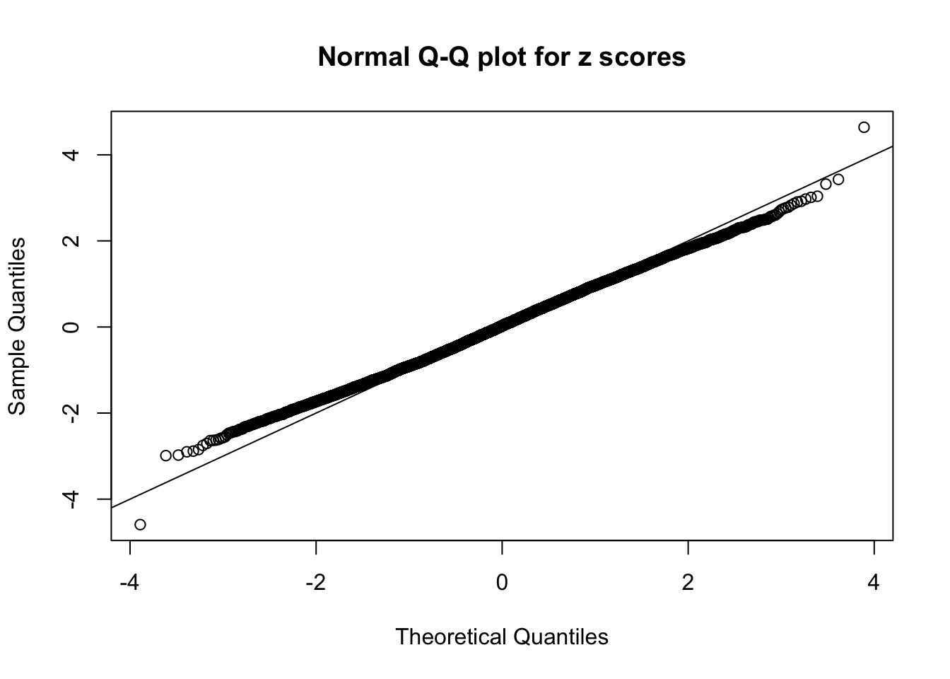
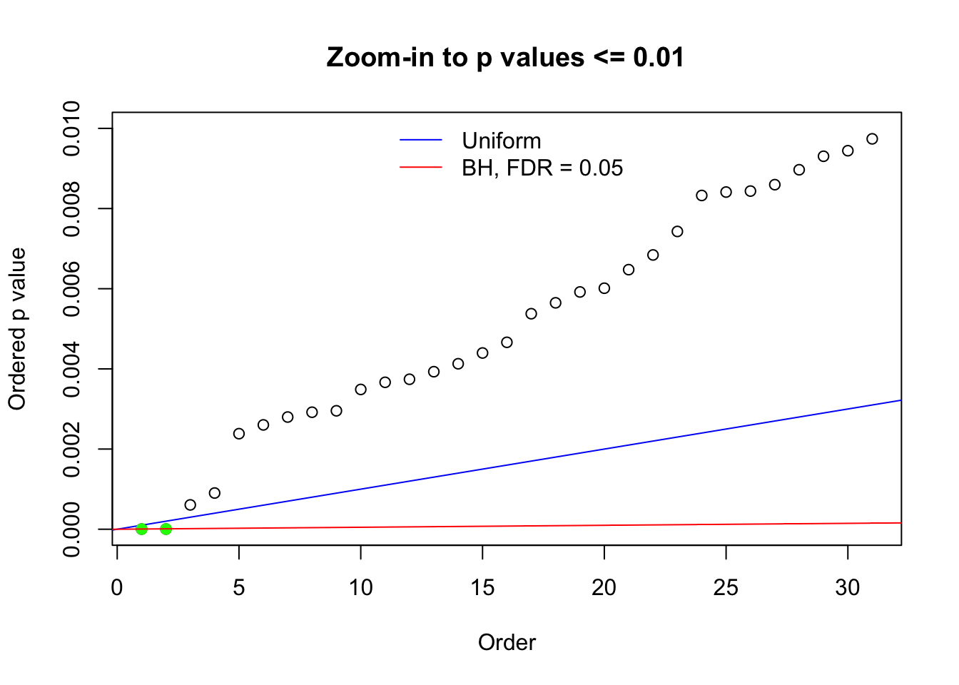
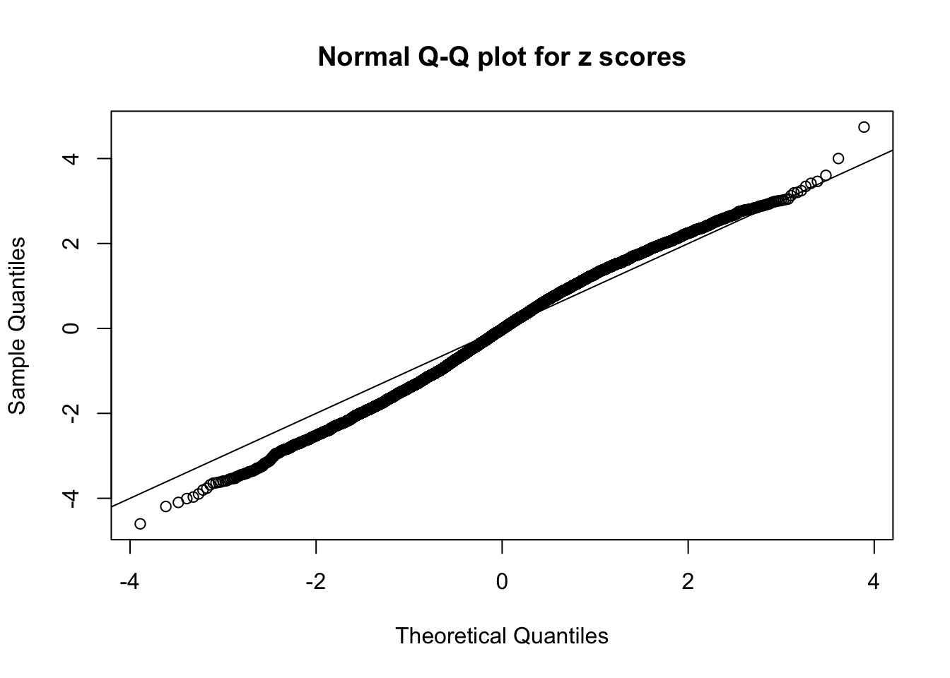
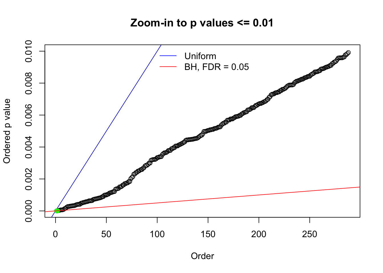
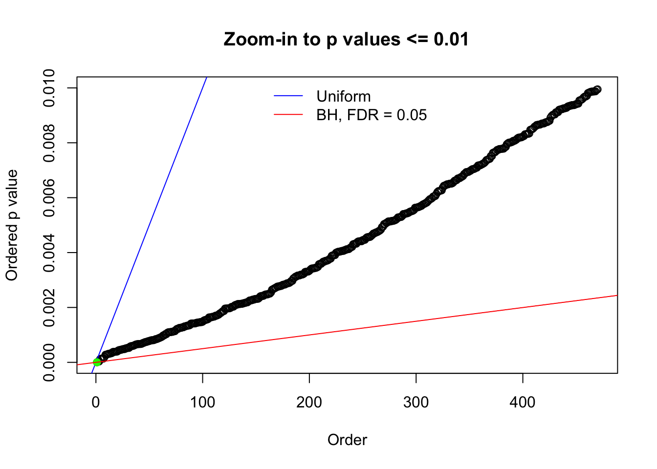
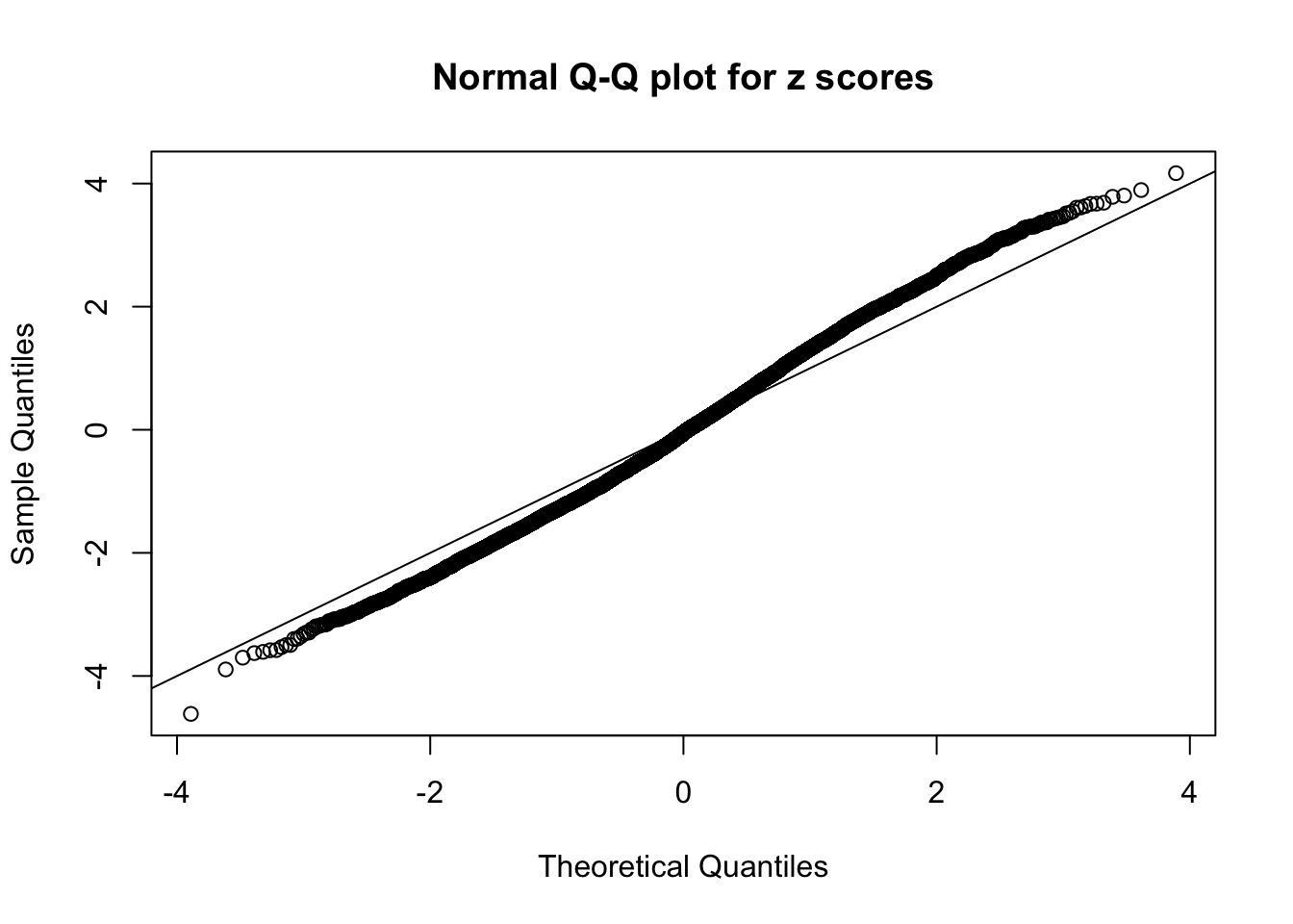
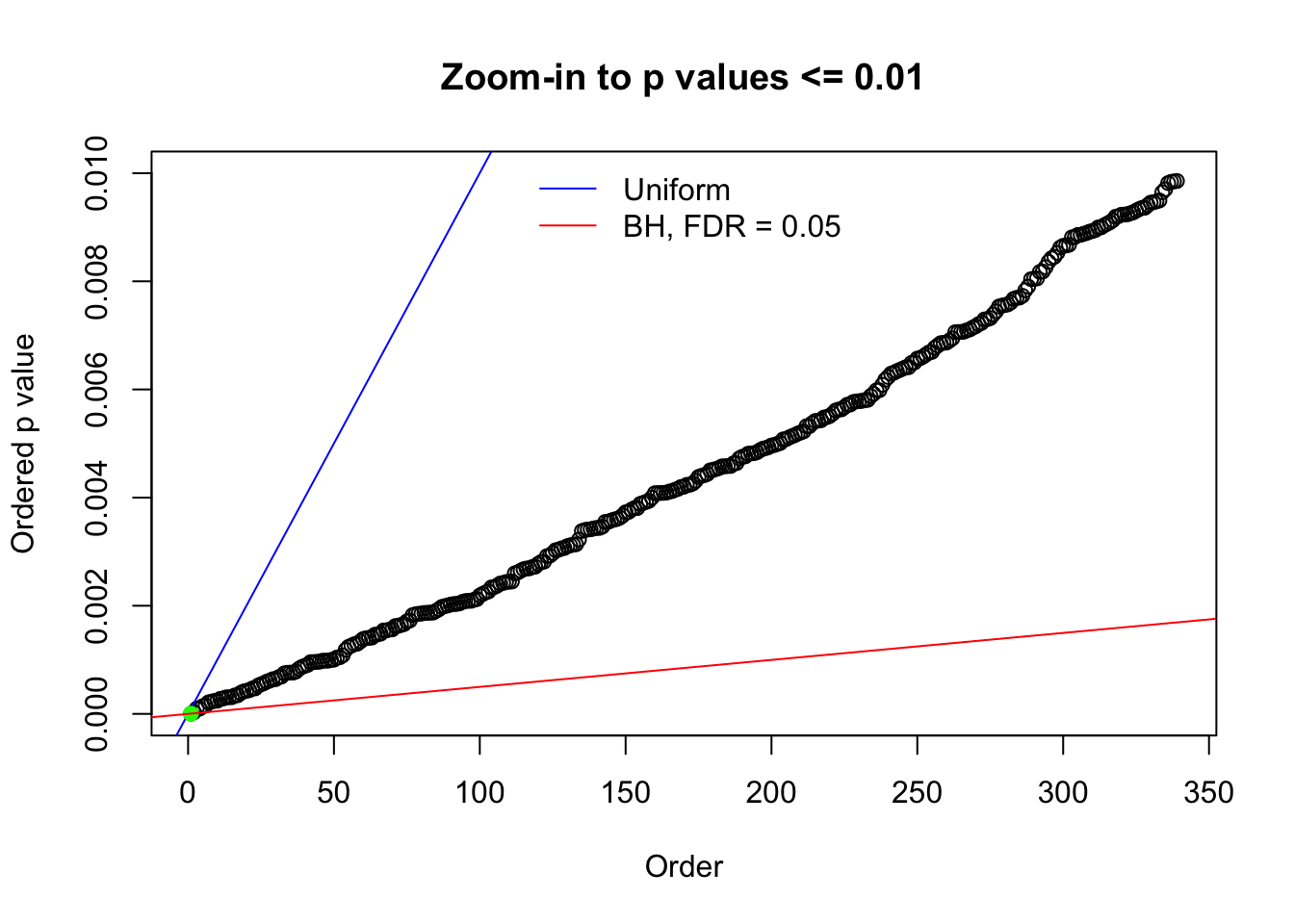
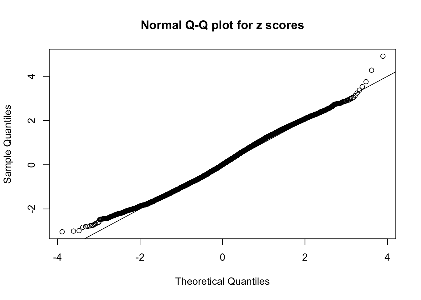
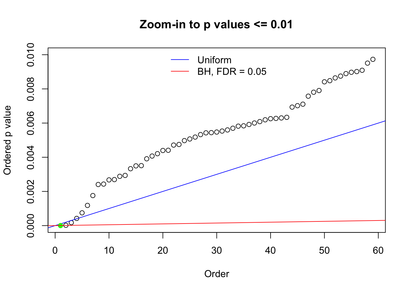
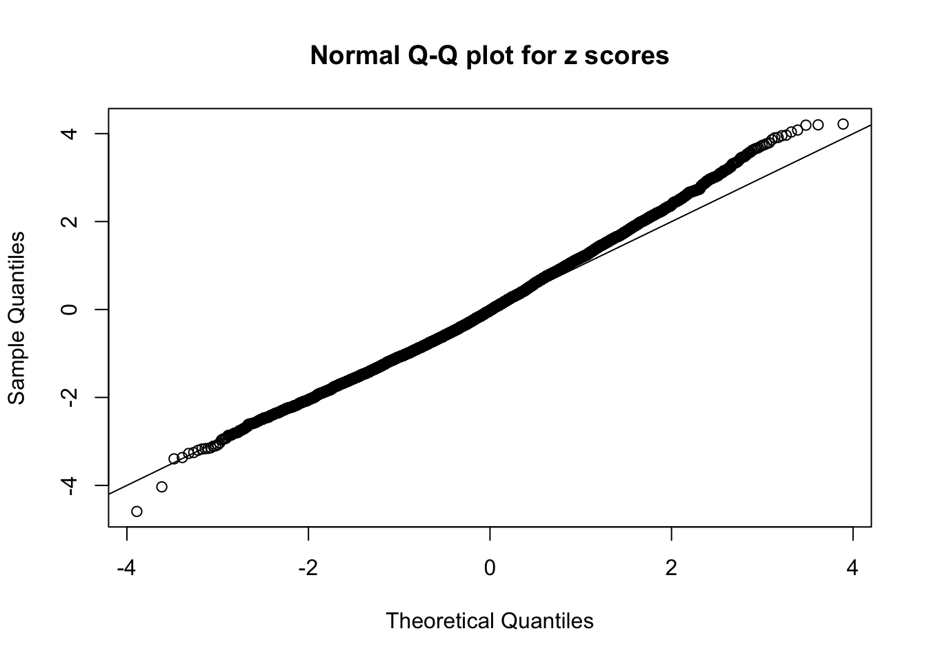
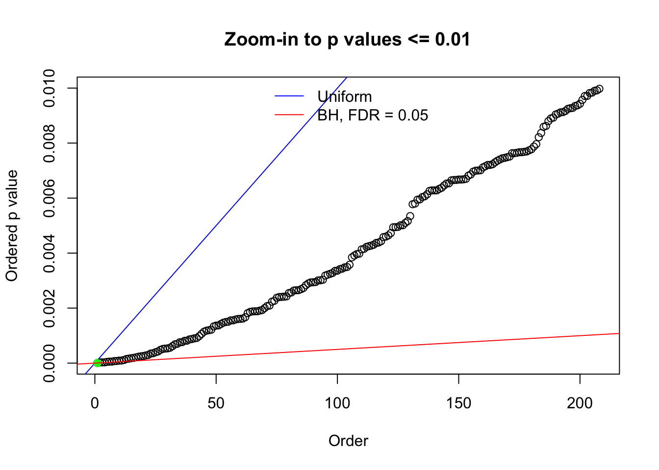
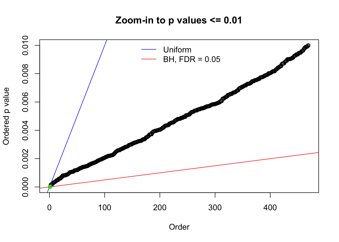
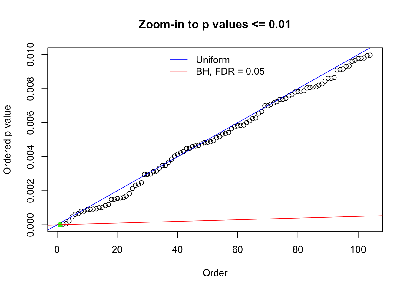
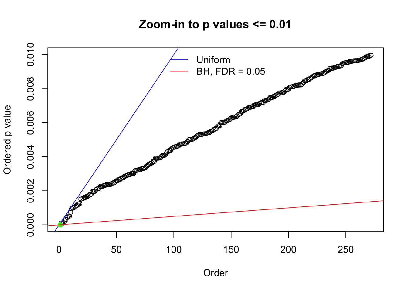
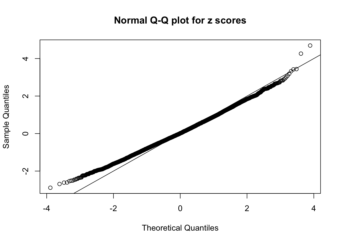
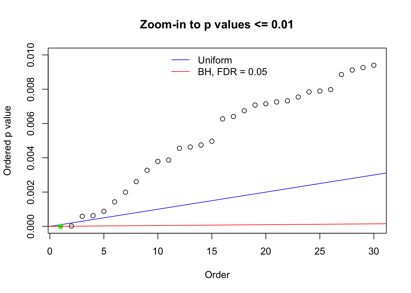
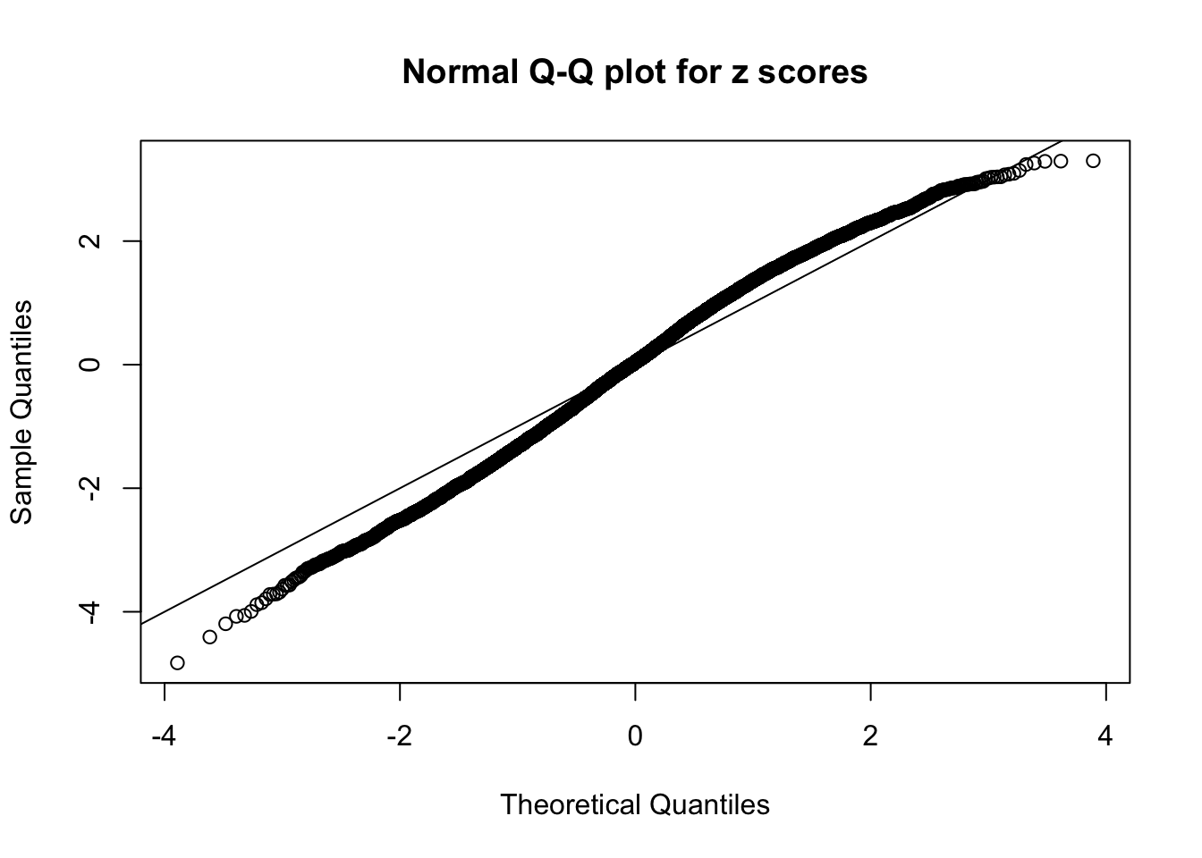
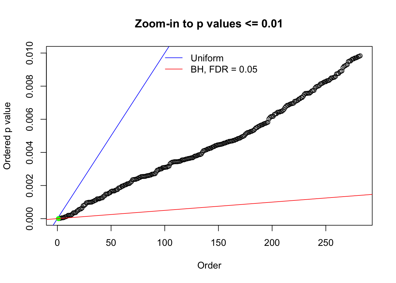
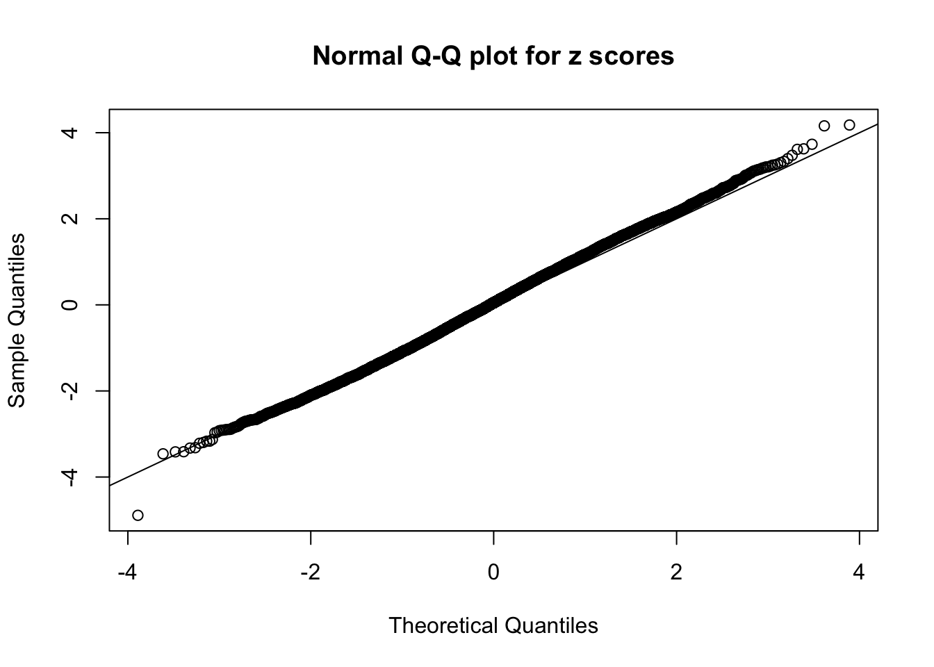
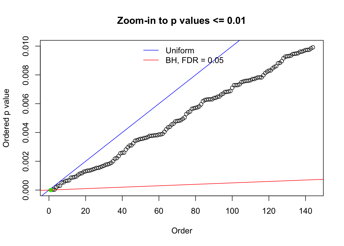
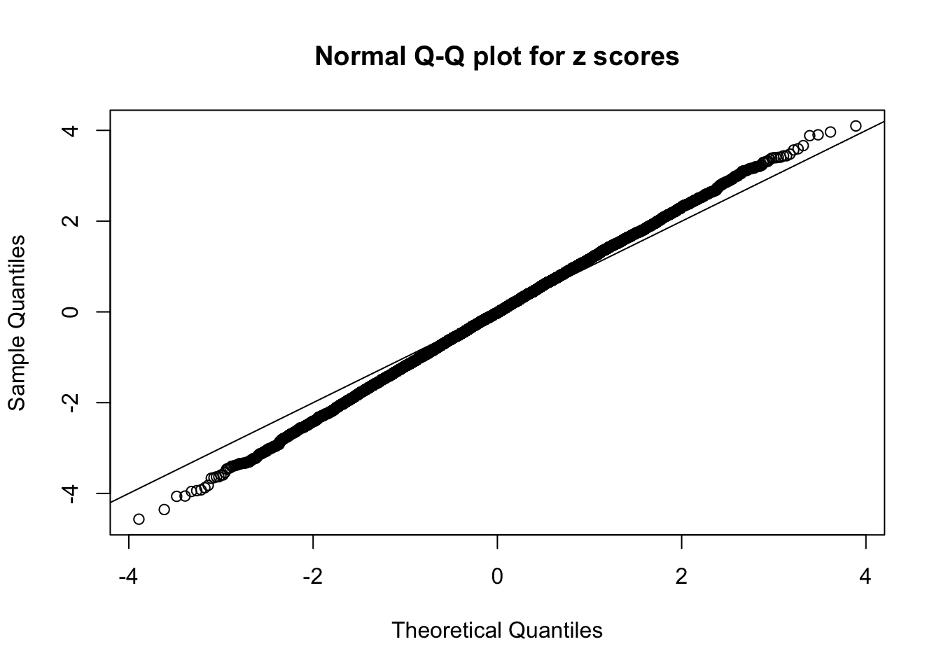
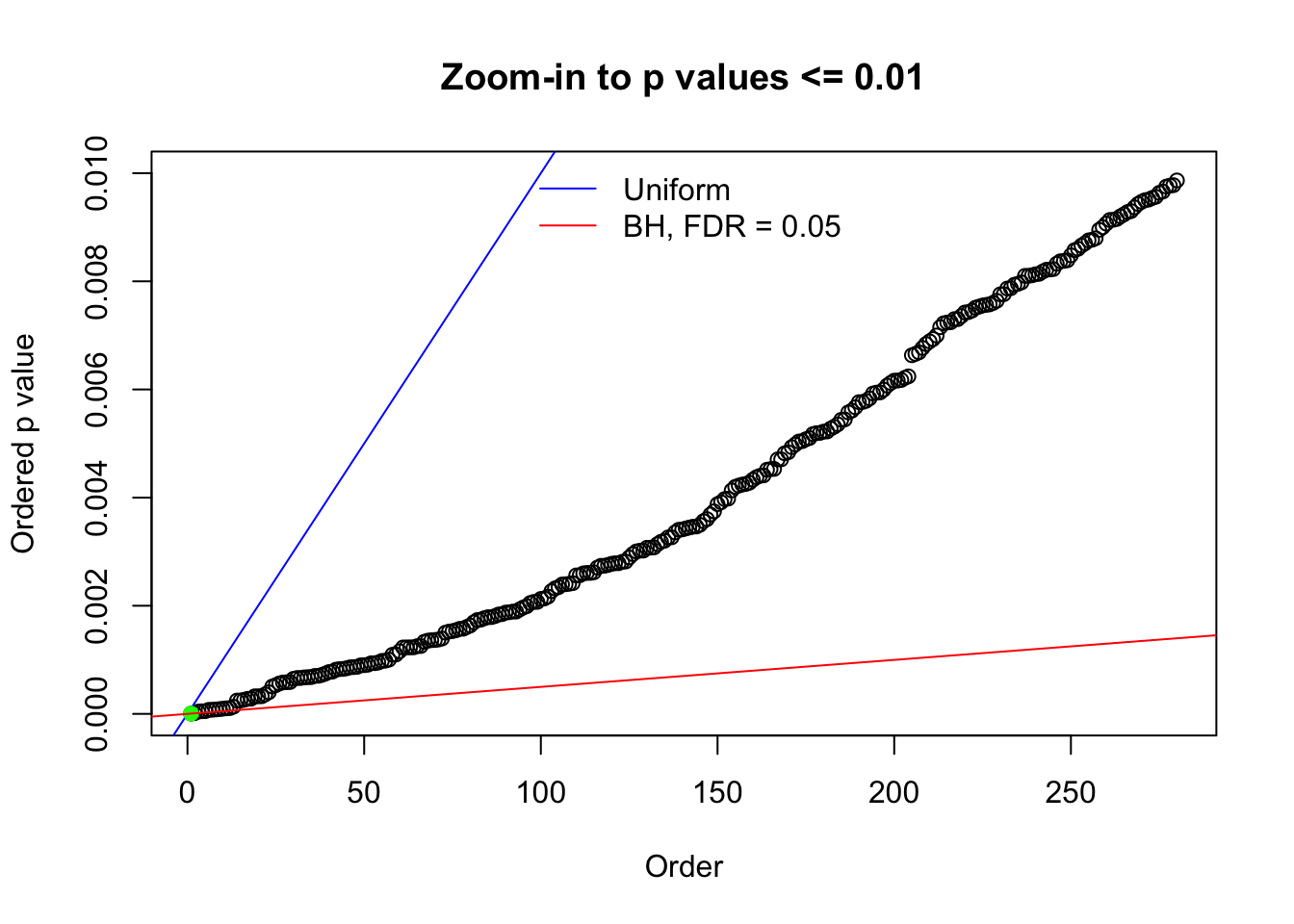
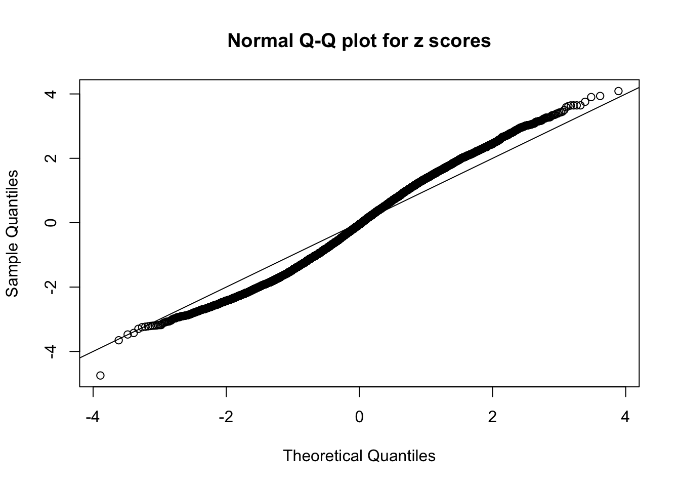
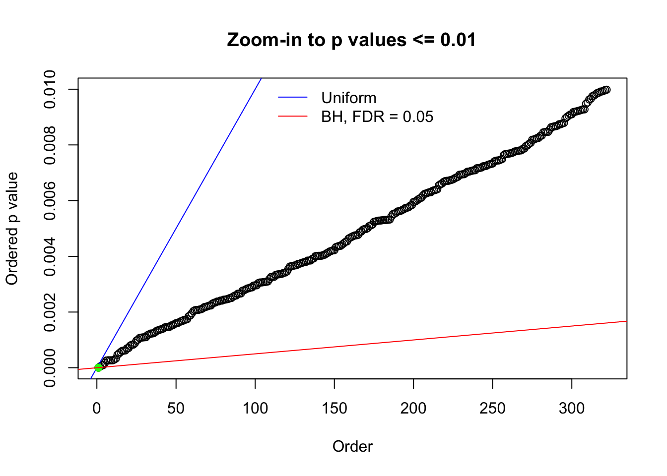
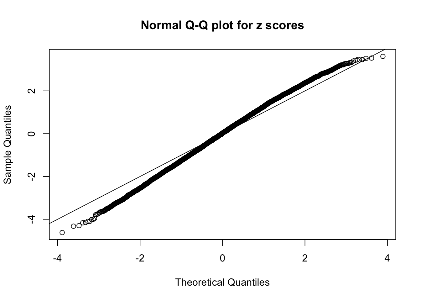
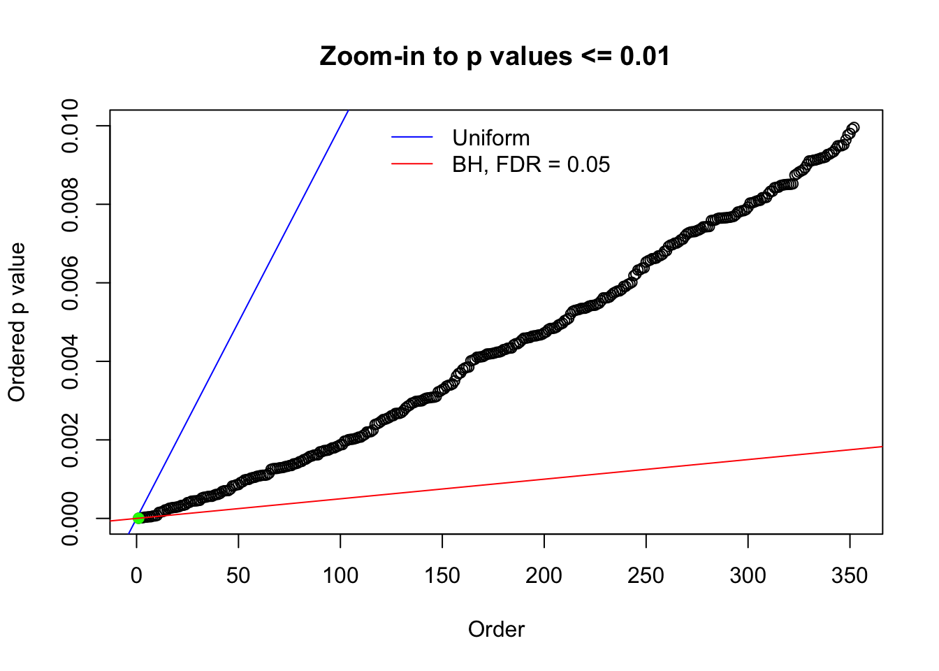
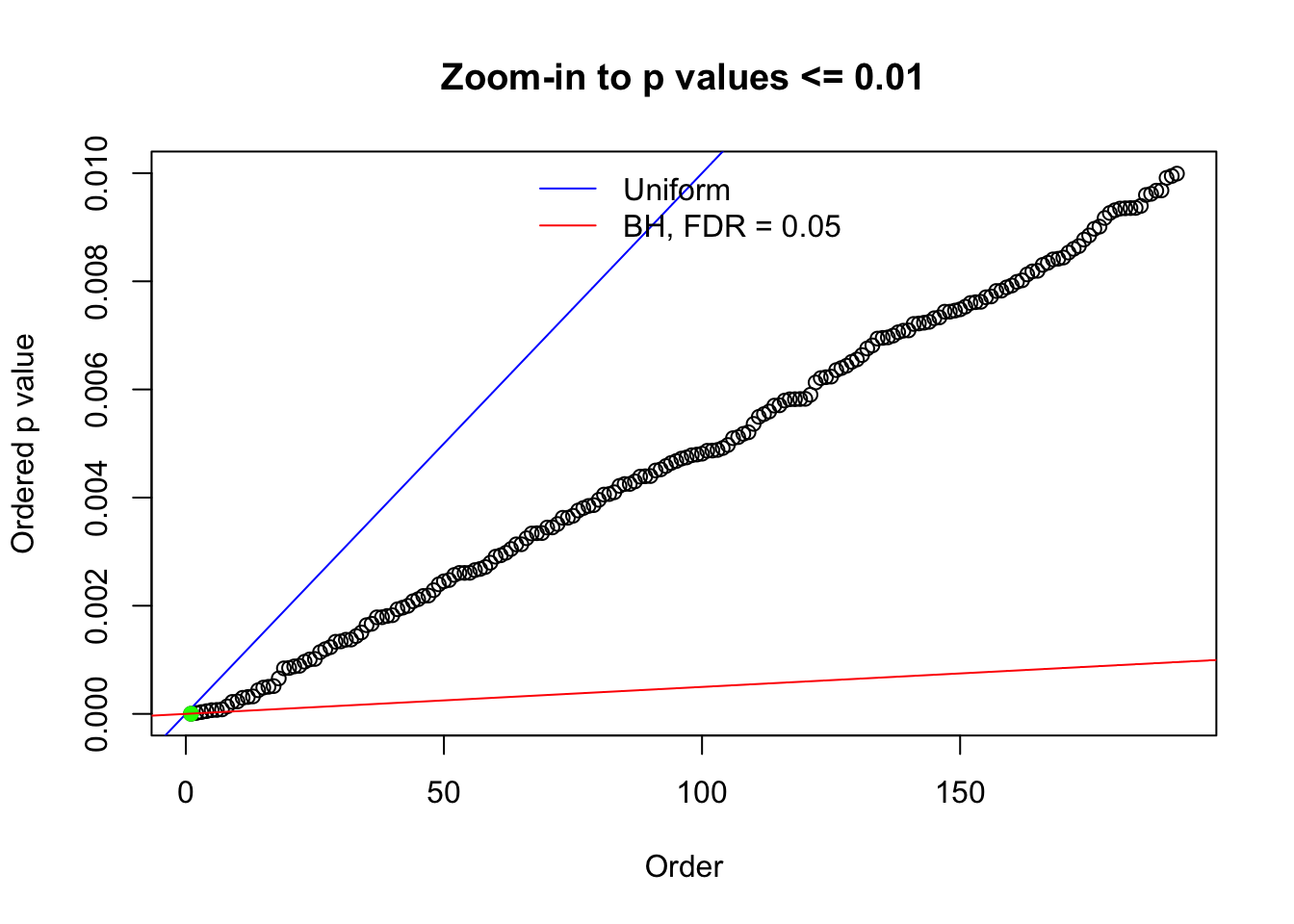
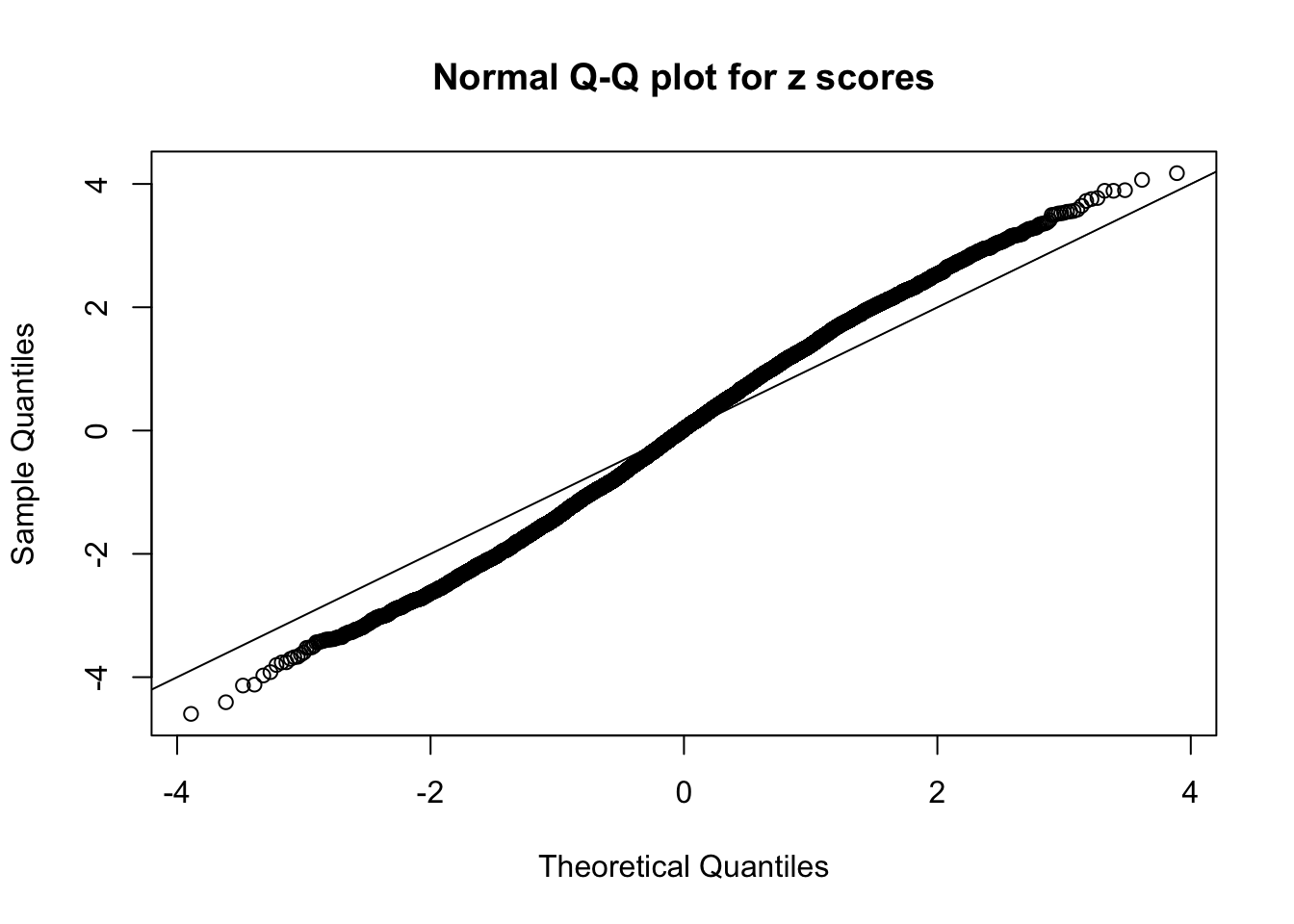
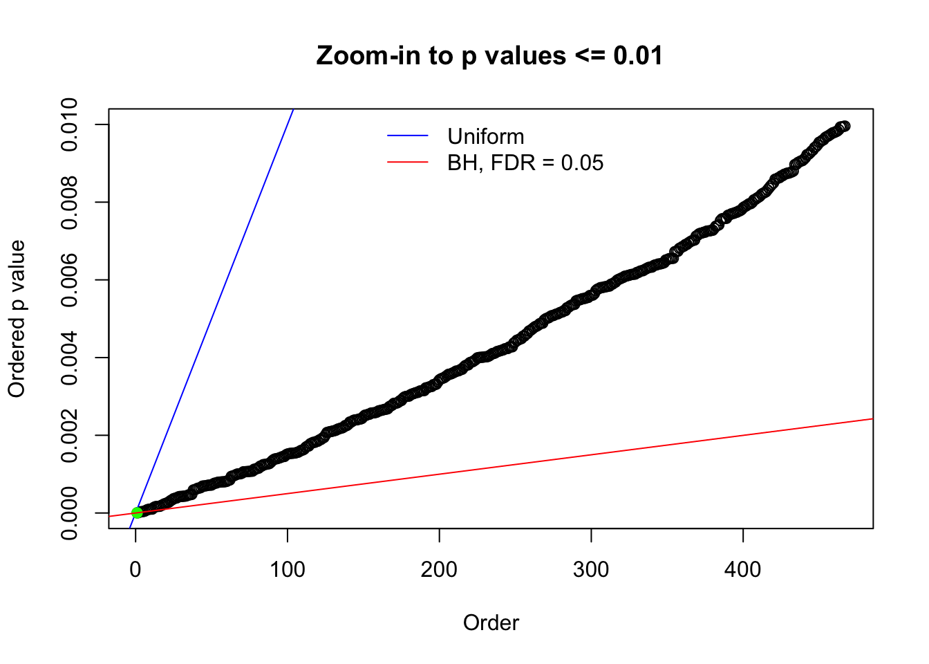
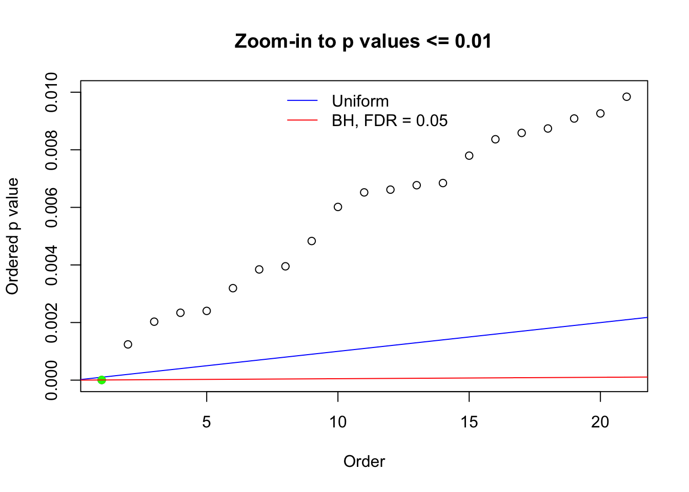
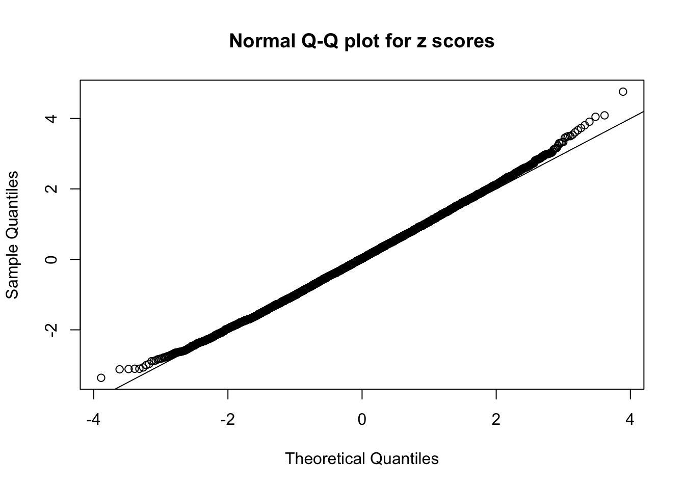
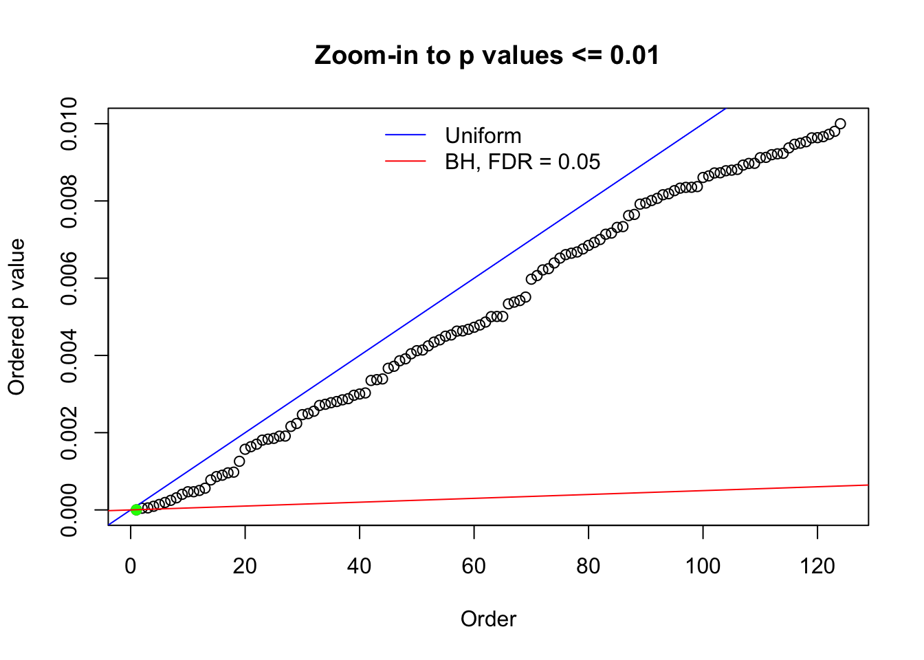
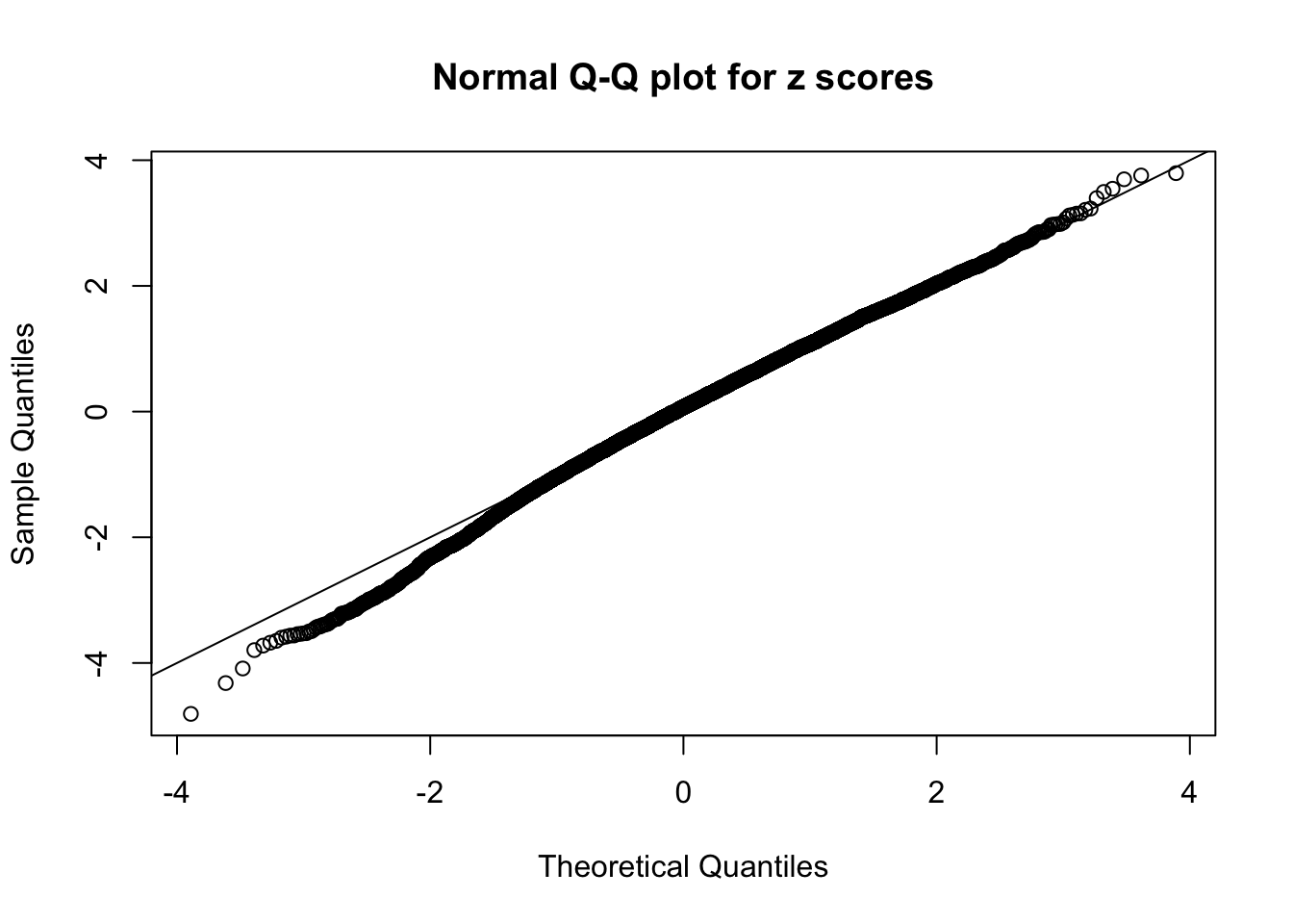
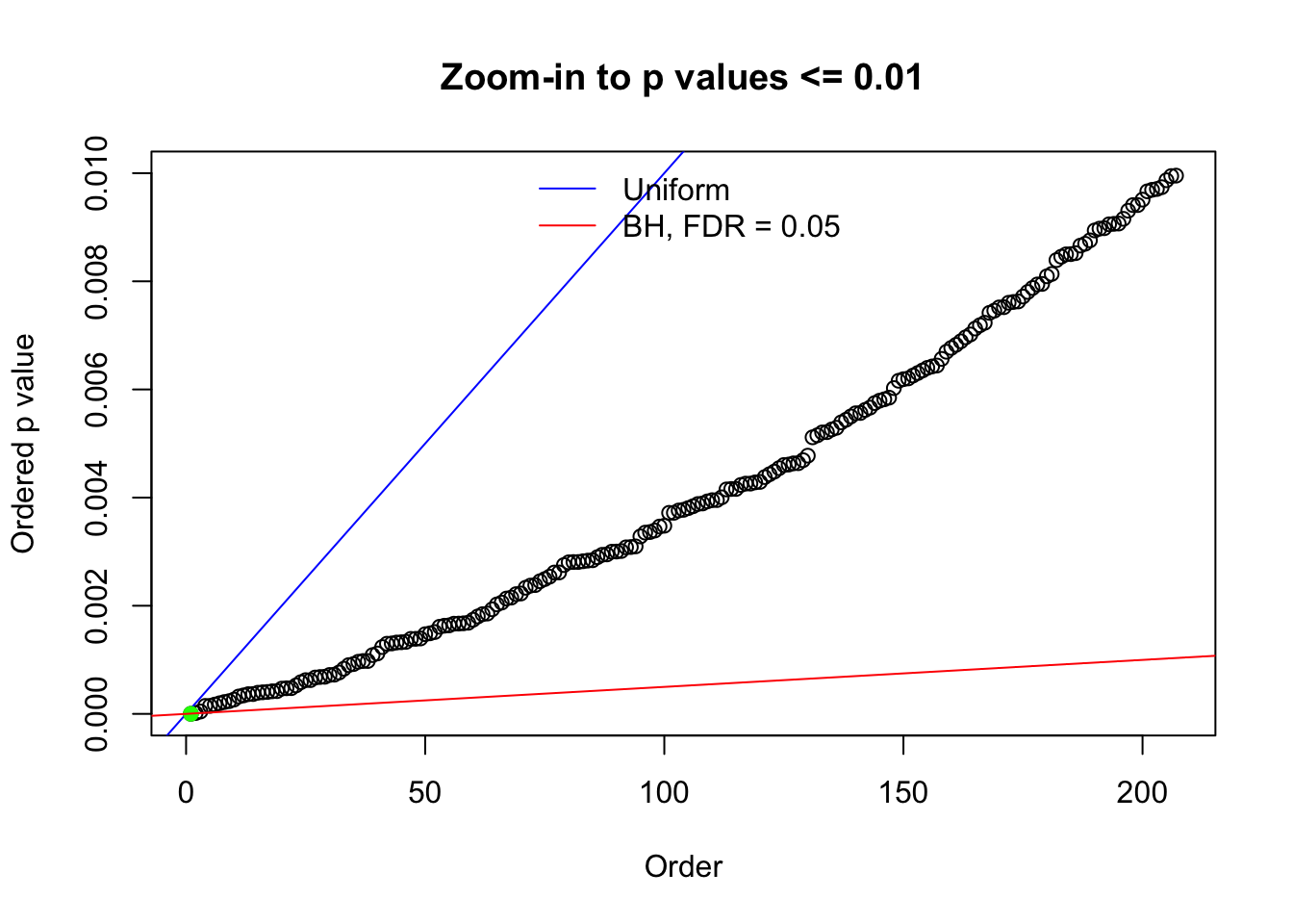
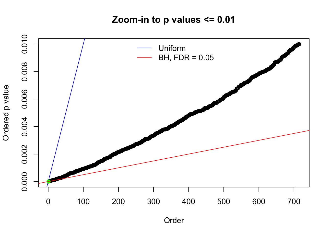
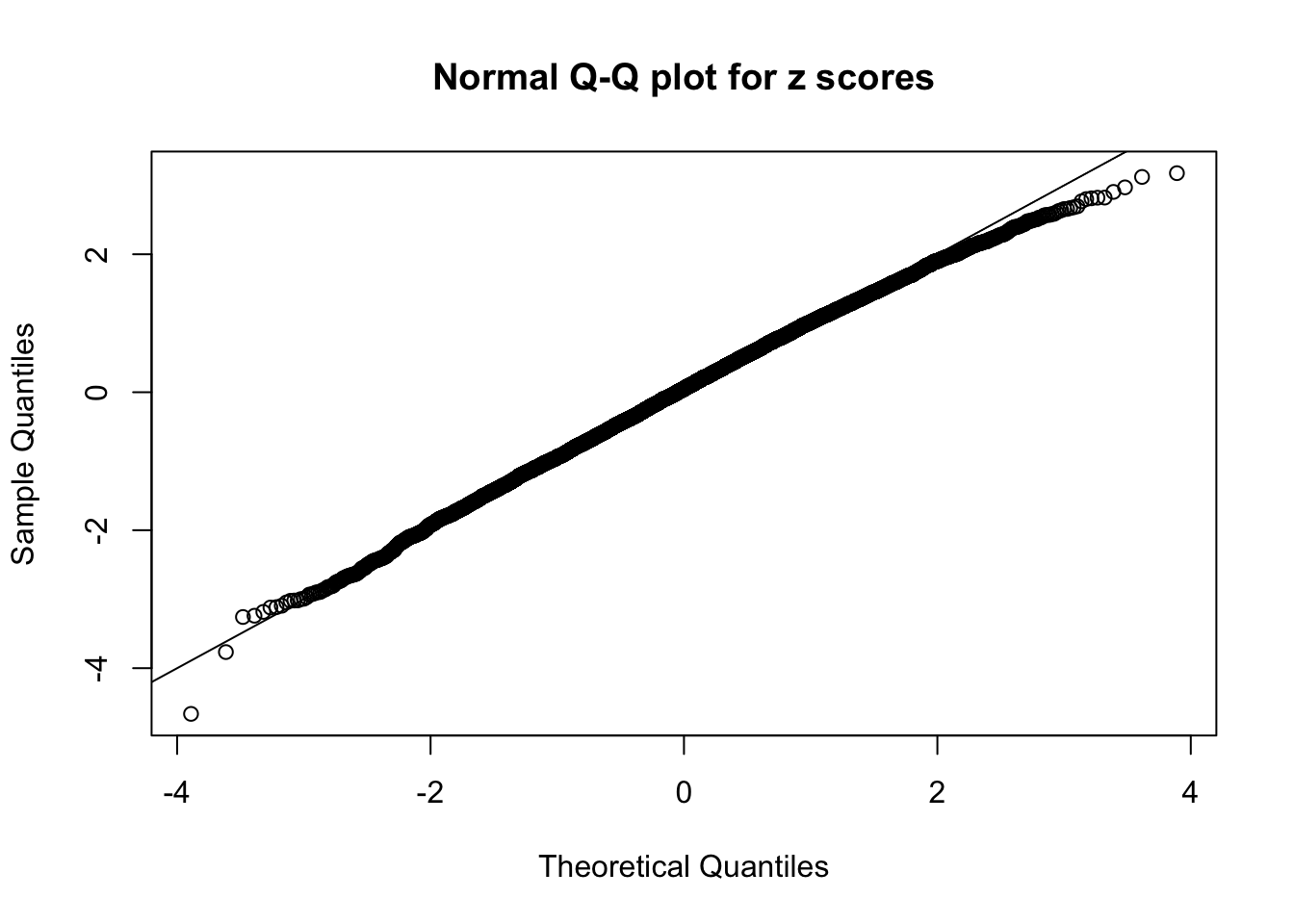
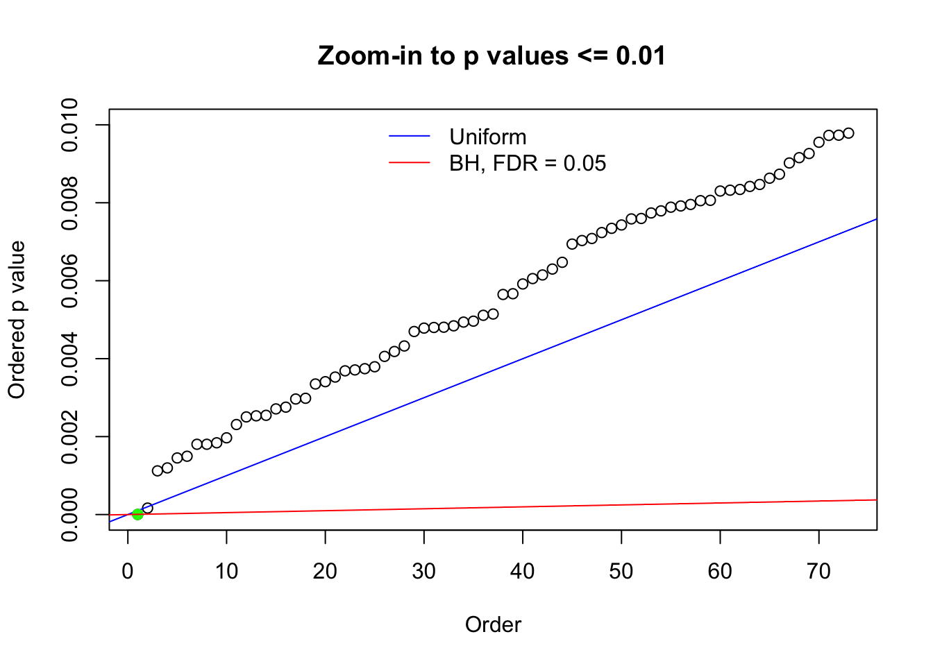
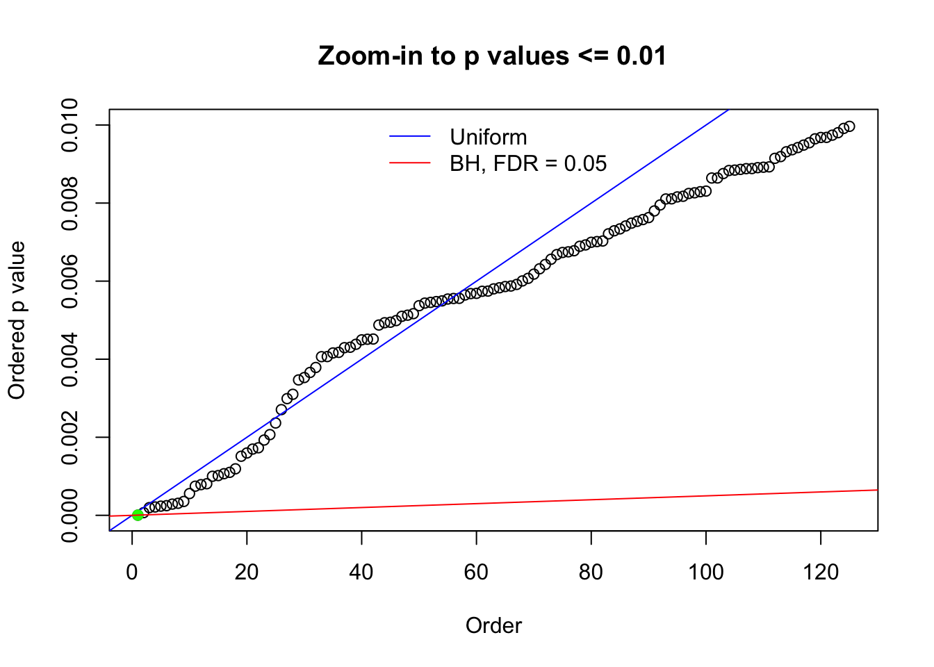
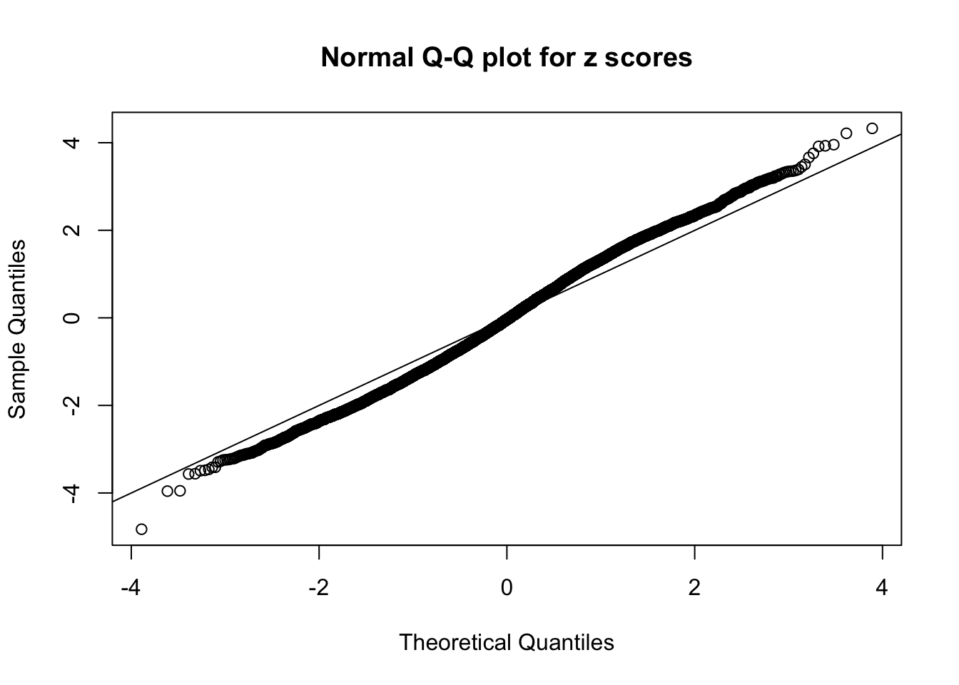
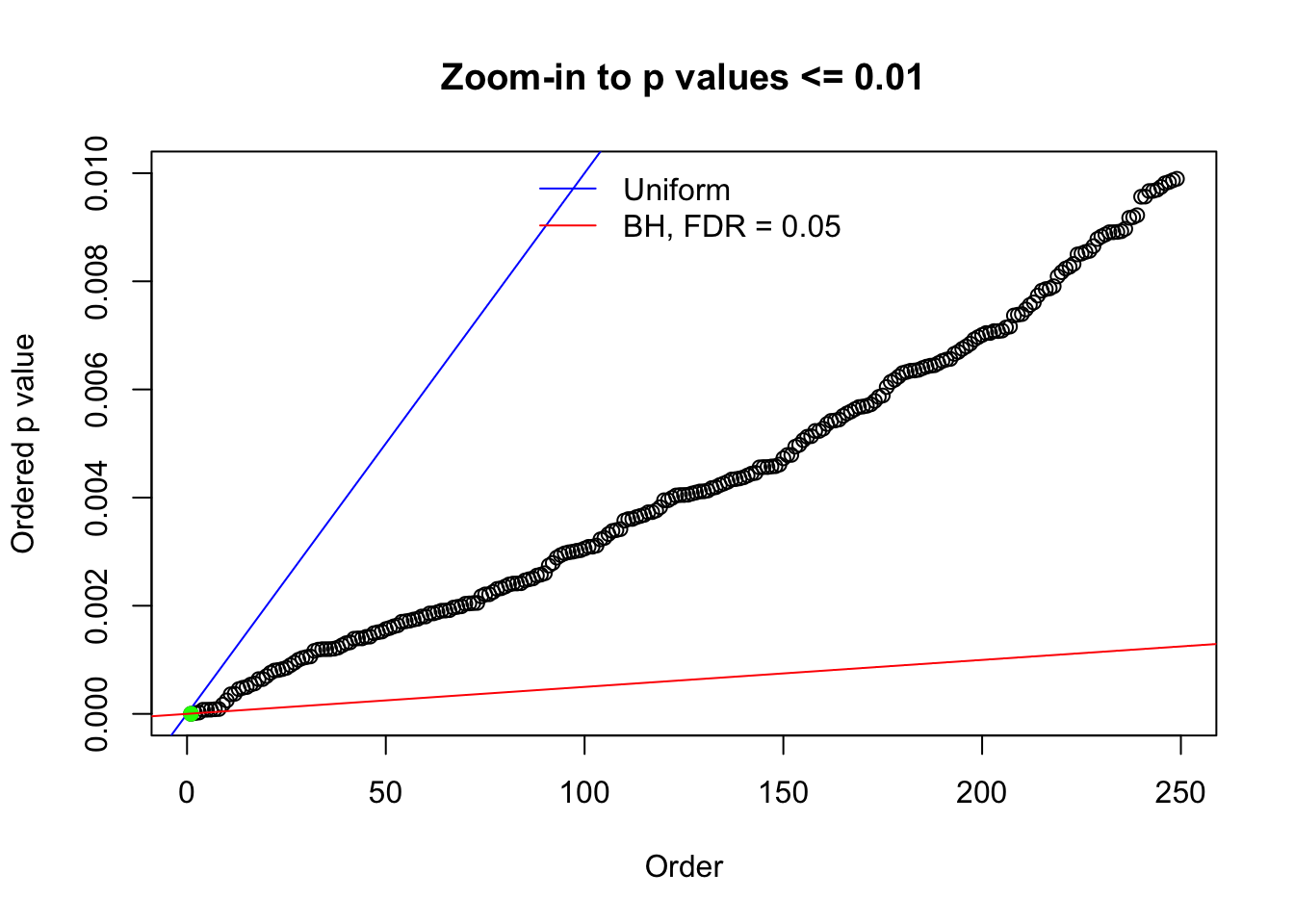
Here we get \(1K\) simulated, correlated null data sets, each having \(10K\) \(z\) scores, \(p\) values associated \(10K\) genes. We choose those data sets most hostile to \(BH\) procedure – those which produce at least false discovery under BH using \(\alpha = 0.05\). And then feed \(\hat\beta_j = z_j, \hat s_j \equiv 1\) to ASH, using a prior of normal mixtures and uniform mixtures, respectively.
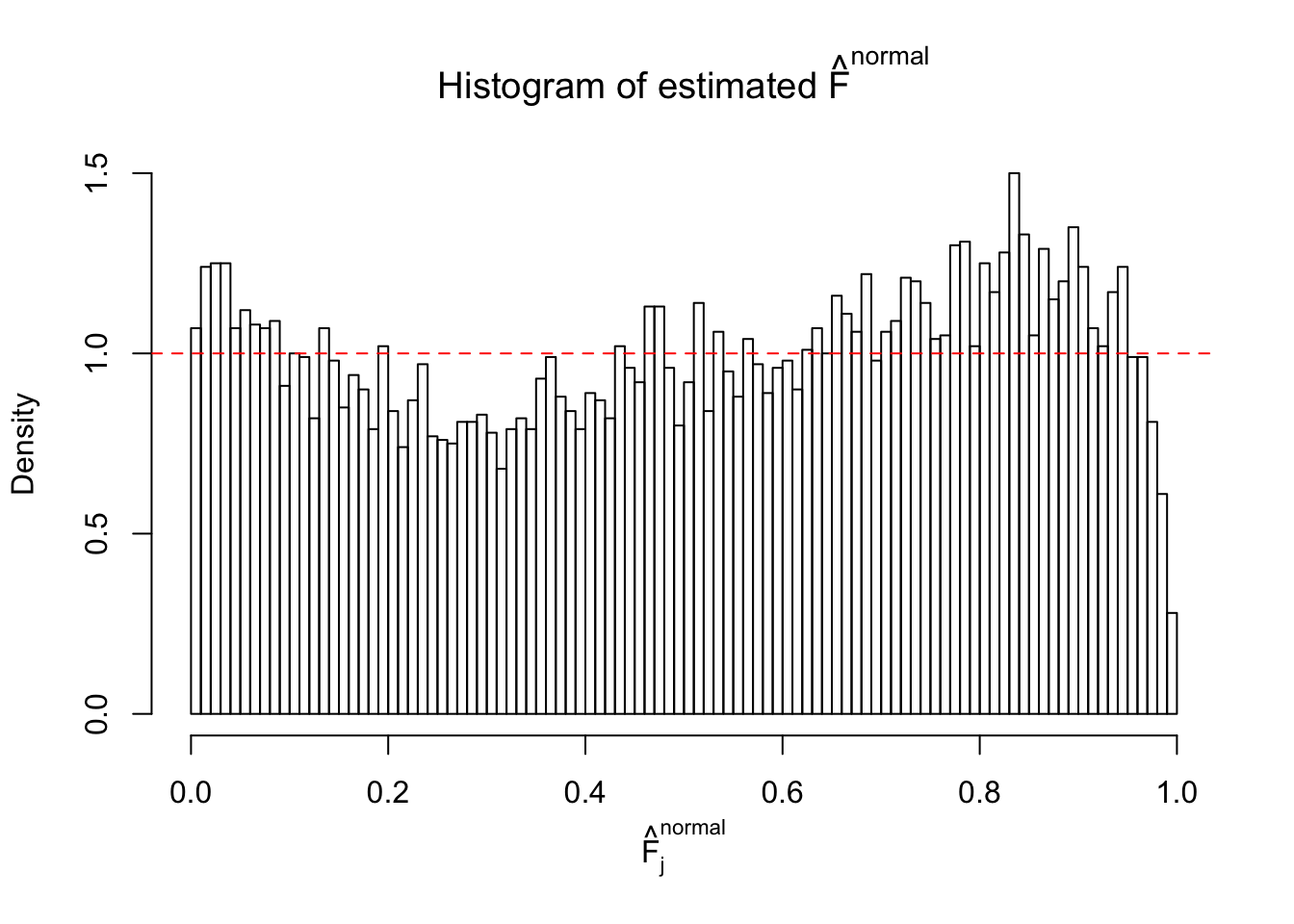
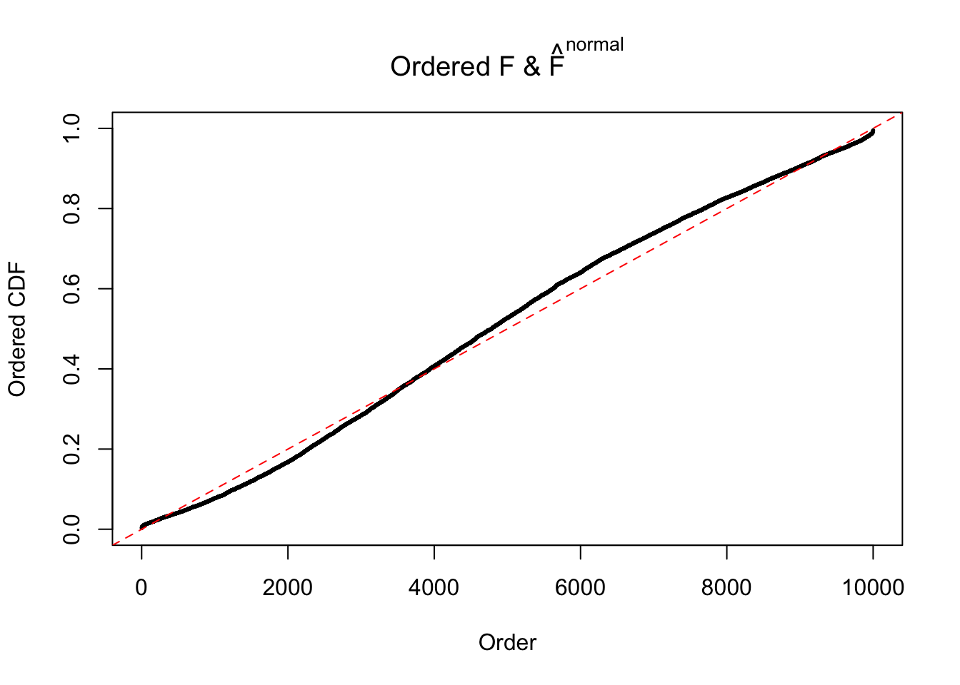
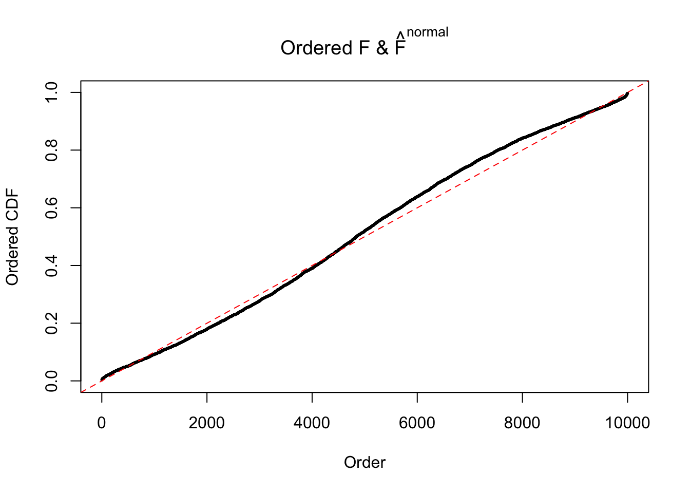
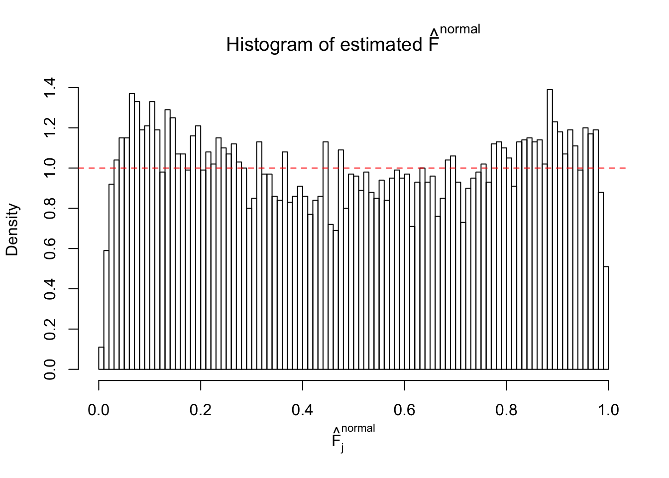
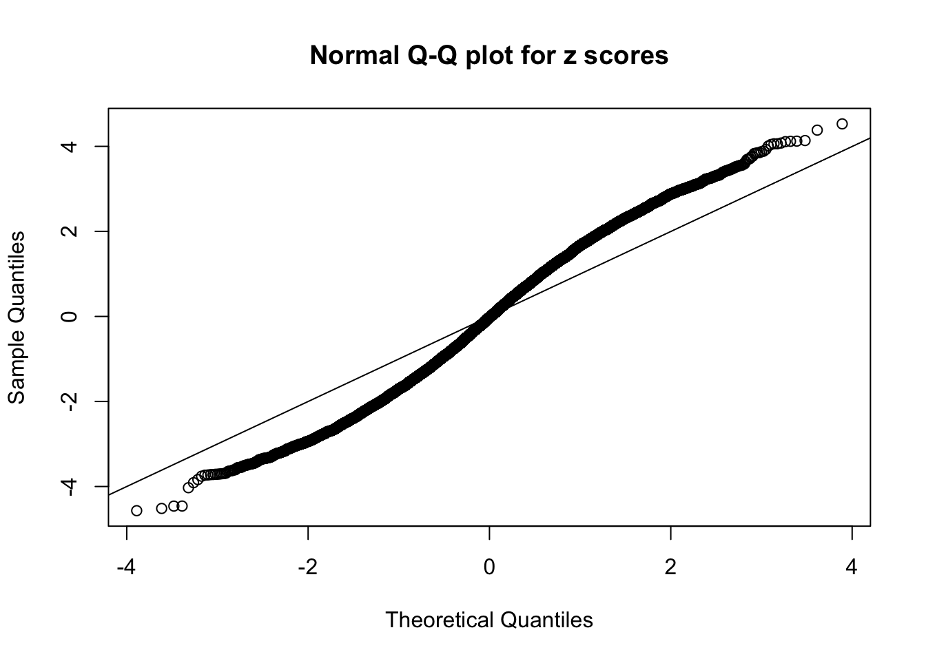
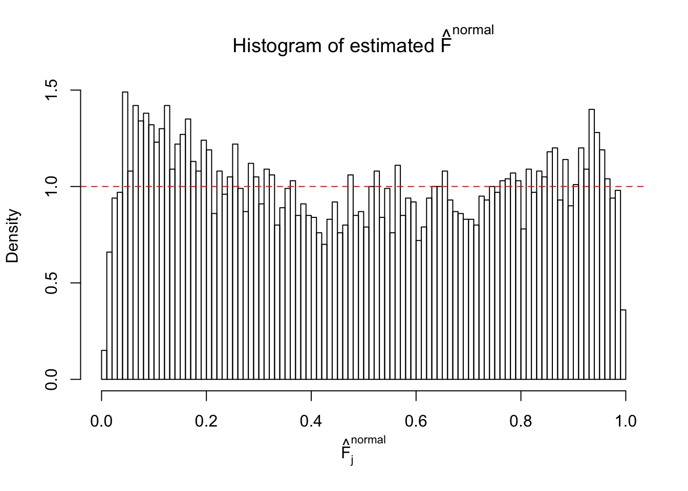
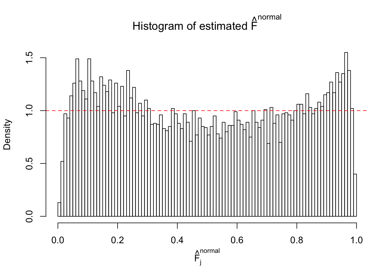
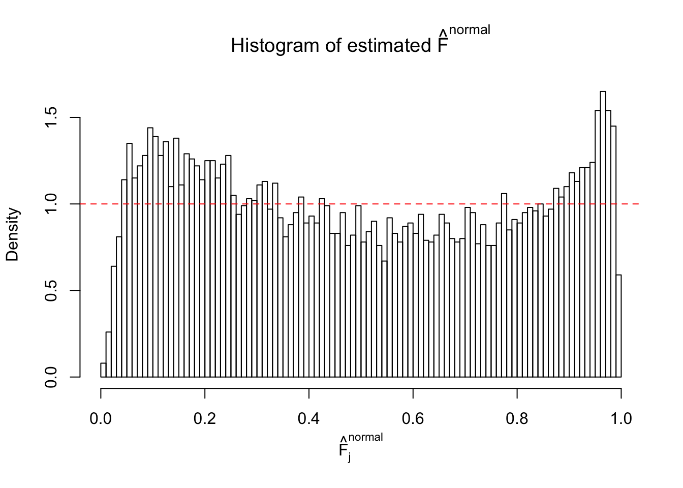
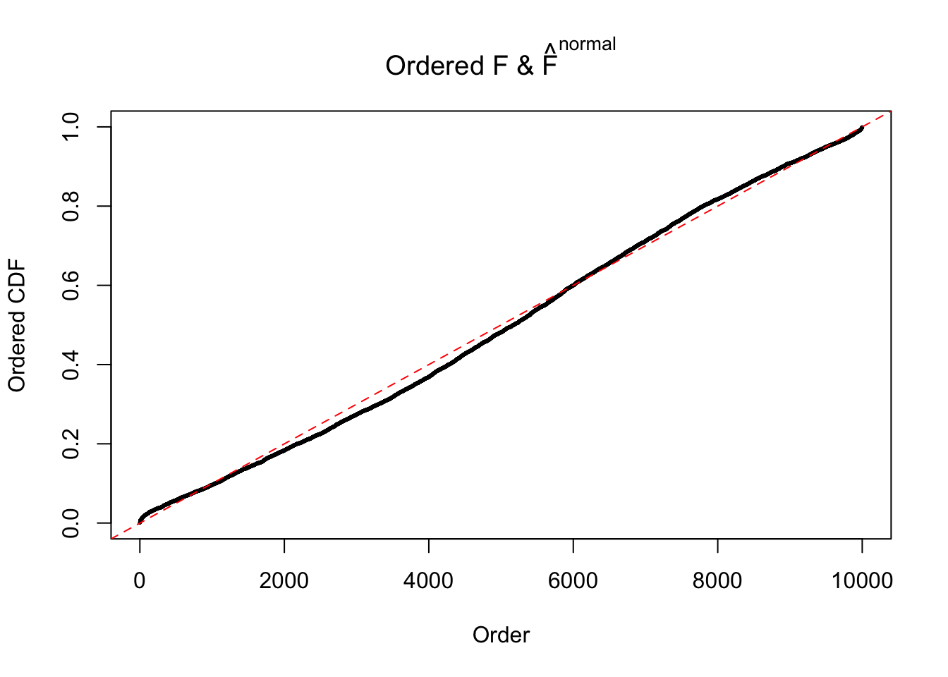
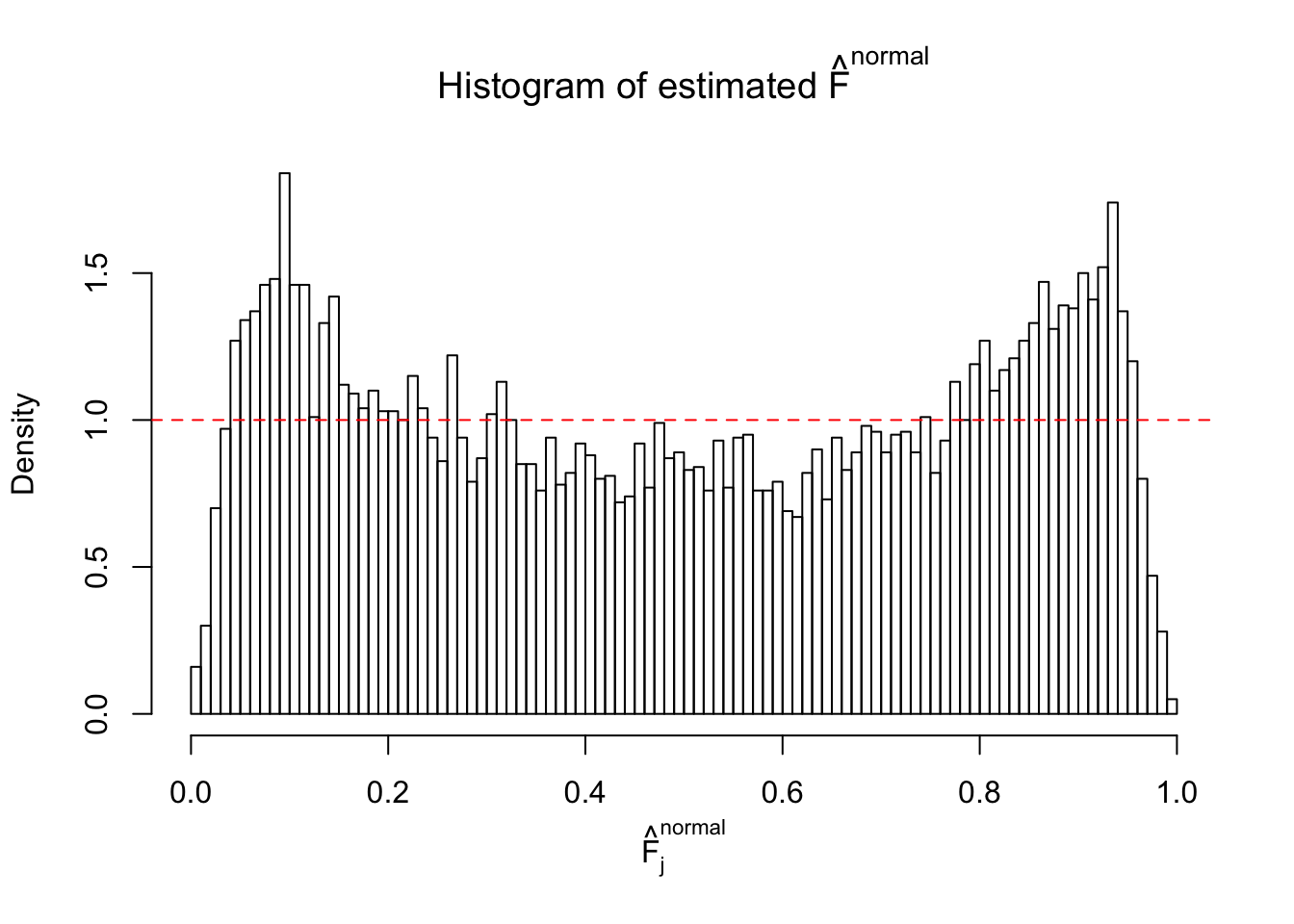
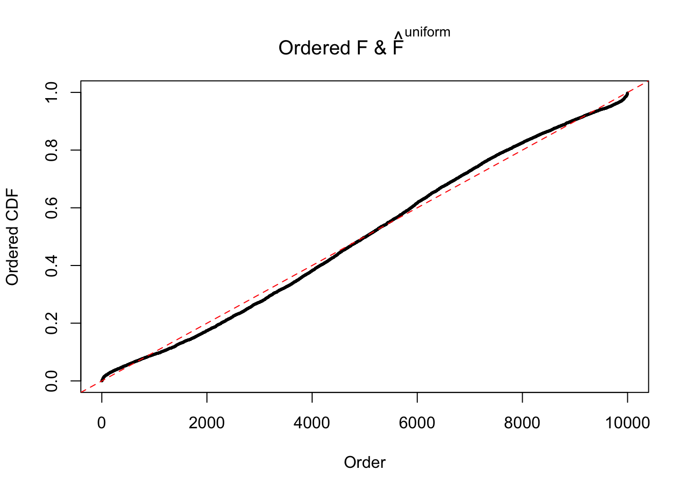
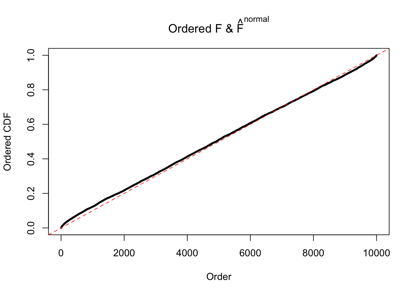
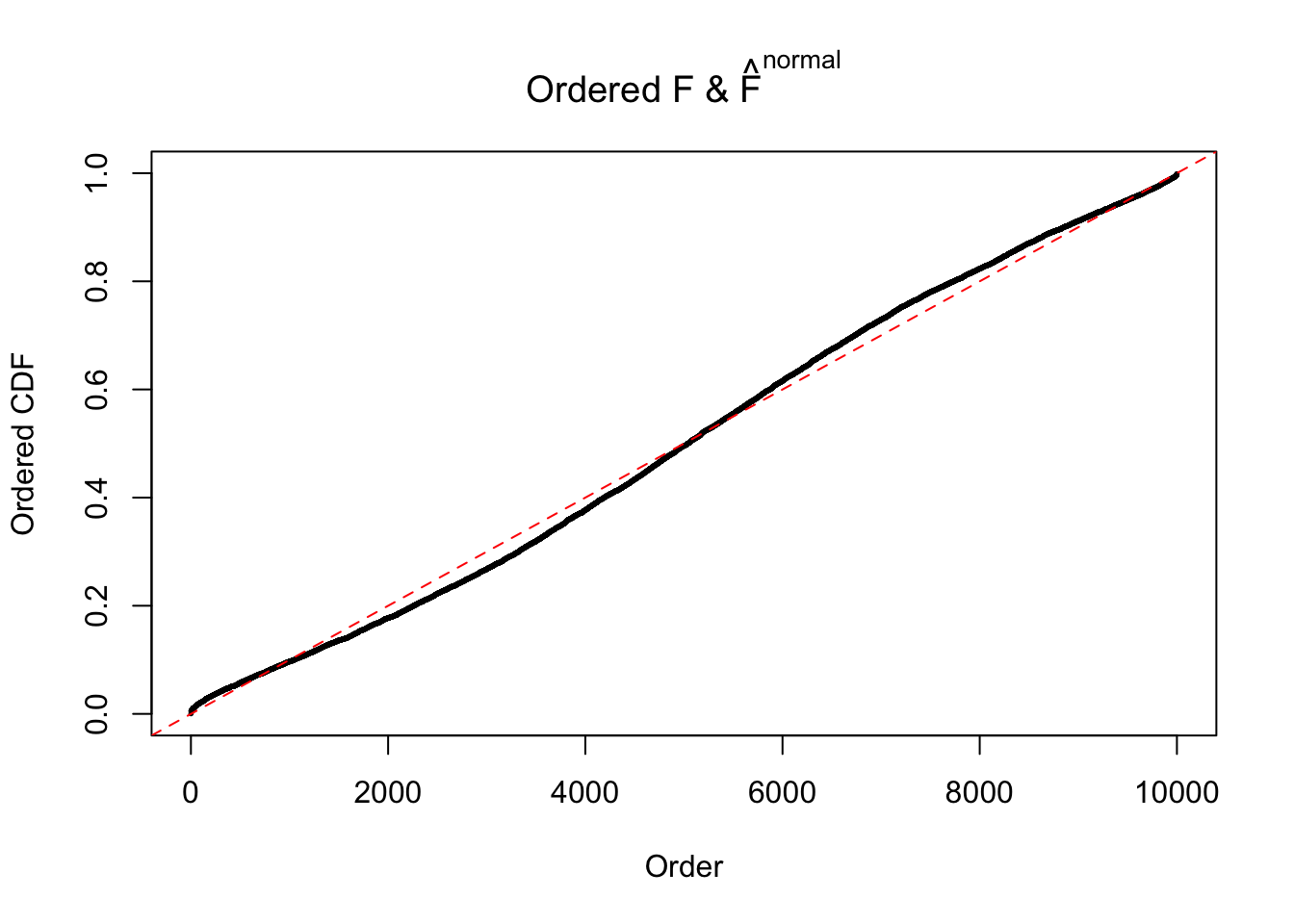
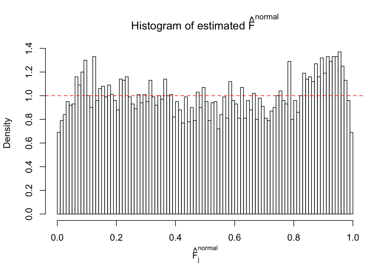
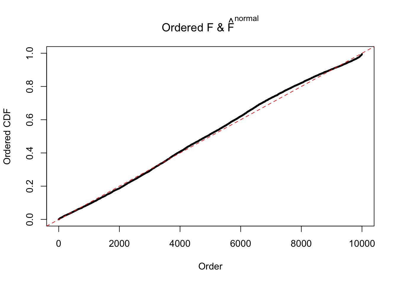
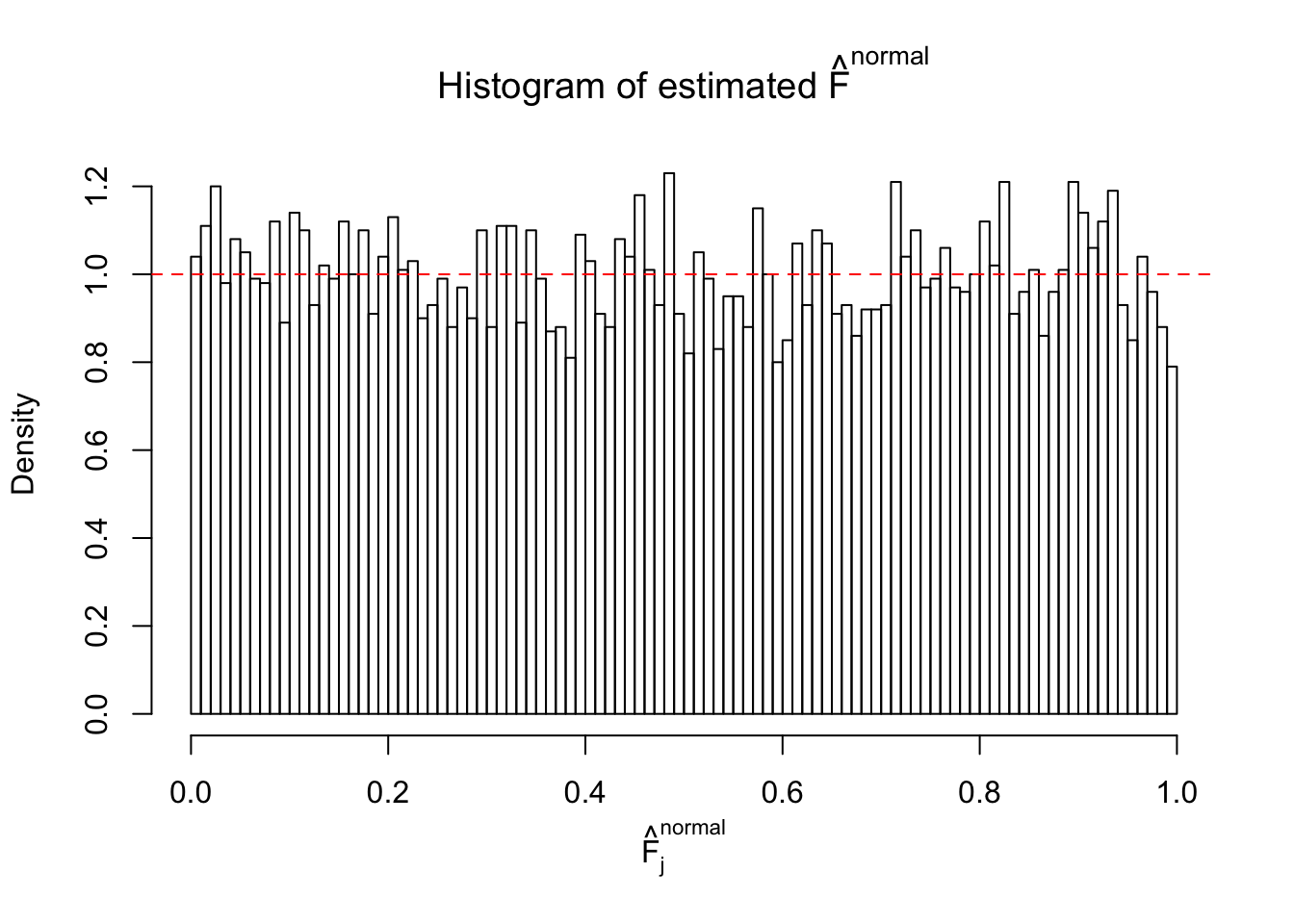
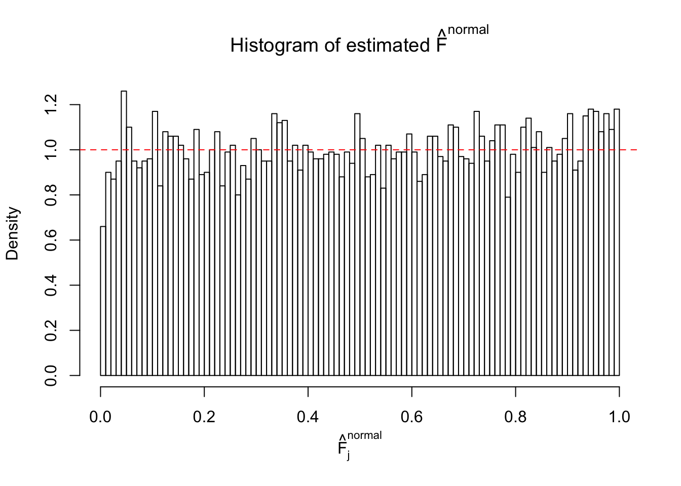
If these \(z\) scores are independent, ASH should be able to estimated \(\hat g =\delta_0\) reasonably well. However, with correlation, estimated \(\hat g\) will be different from \(\delta_0\). Moreover, with this estimated \(\hat g\), \(\left\{\hat F_j\right\}\) might not behave like \(\text{Unif}\left[0, 1\right]\).
This is because the pseudo-effect due to the correlation-induced inflation is not regular and not likely to be captured by unimodal mixtures of normals of uniforms. For example, as Matthew’s initial observation which inspired the whole project in the first place, the correlation may only inflate the moderate observations but not the extreme ones. Thus, a mixture of normals, which simultaneously inflates both the moderate and the extreme observations, would be ill-advised.
library(ashr)z = read.table("../output/z_null_liver_777.txt")
p = read.table("../output/p_null_liver_777.txt")
n = nrow(z)
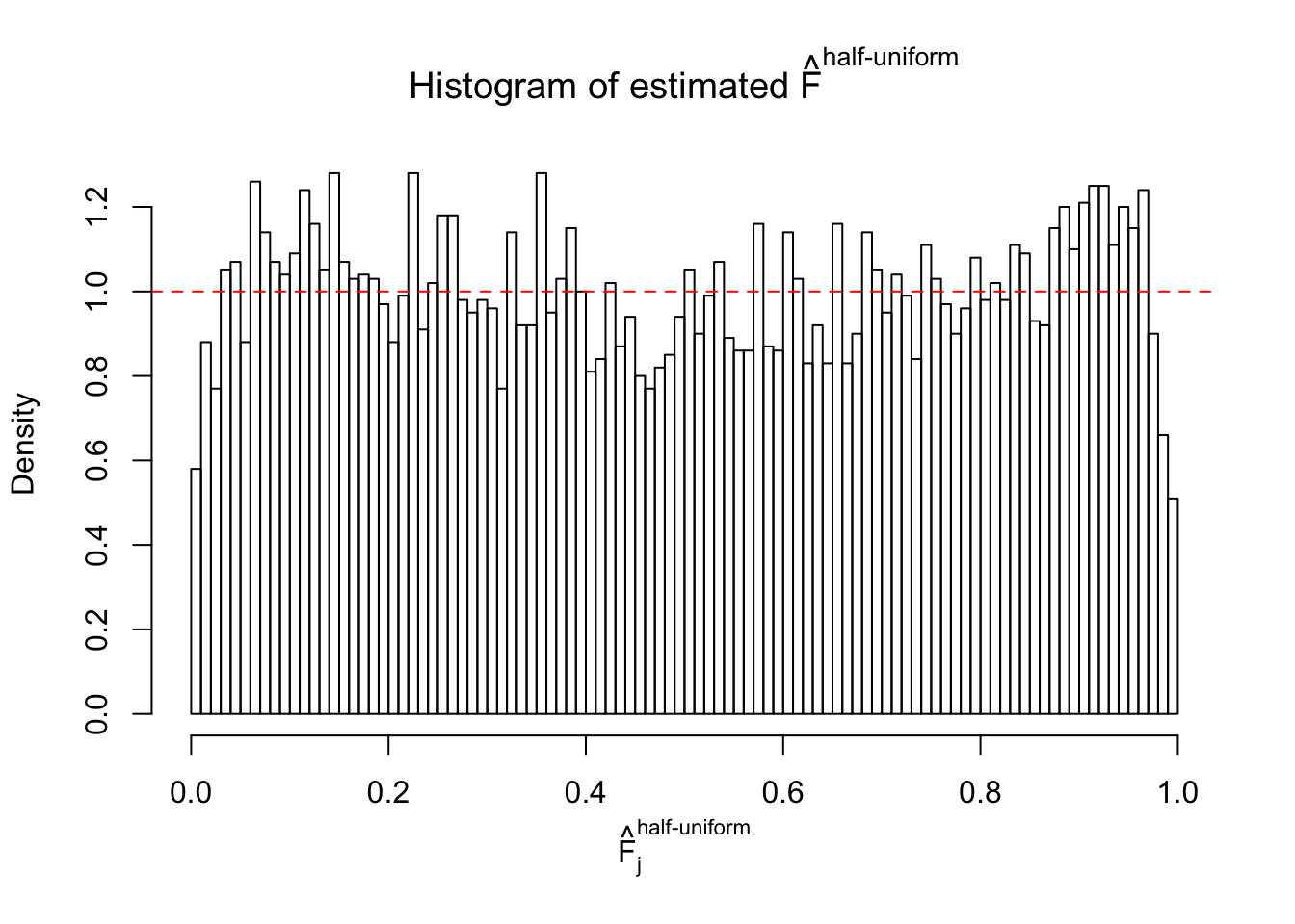
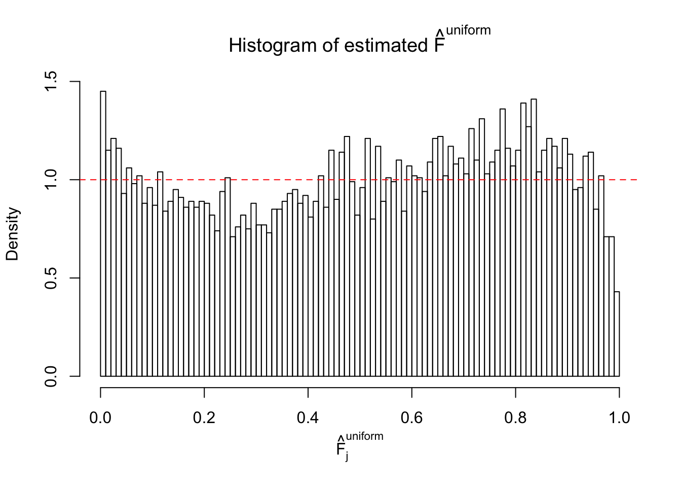
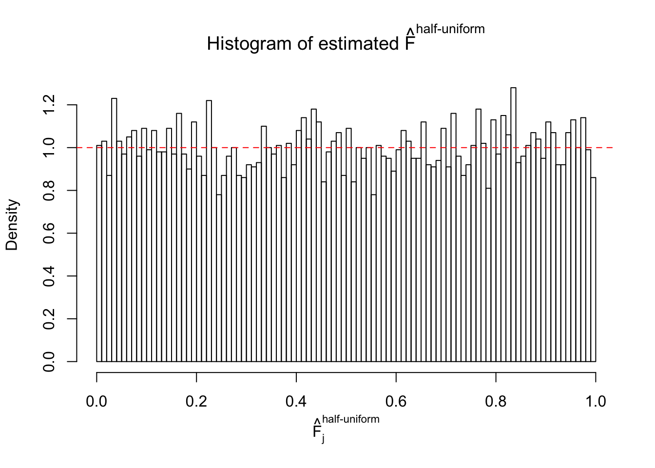
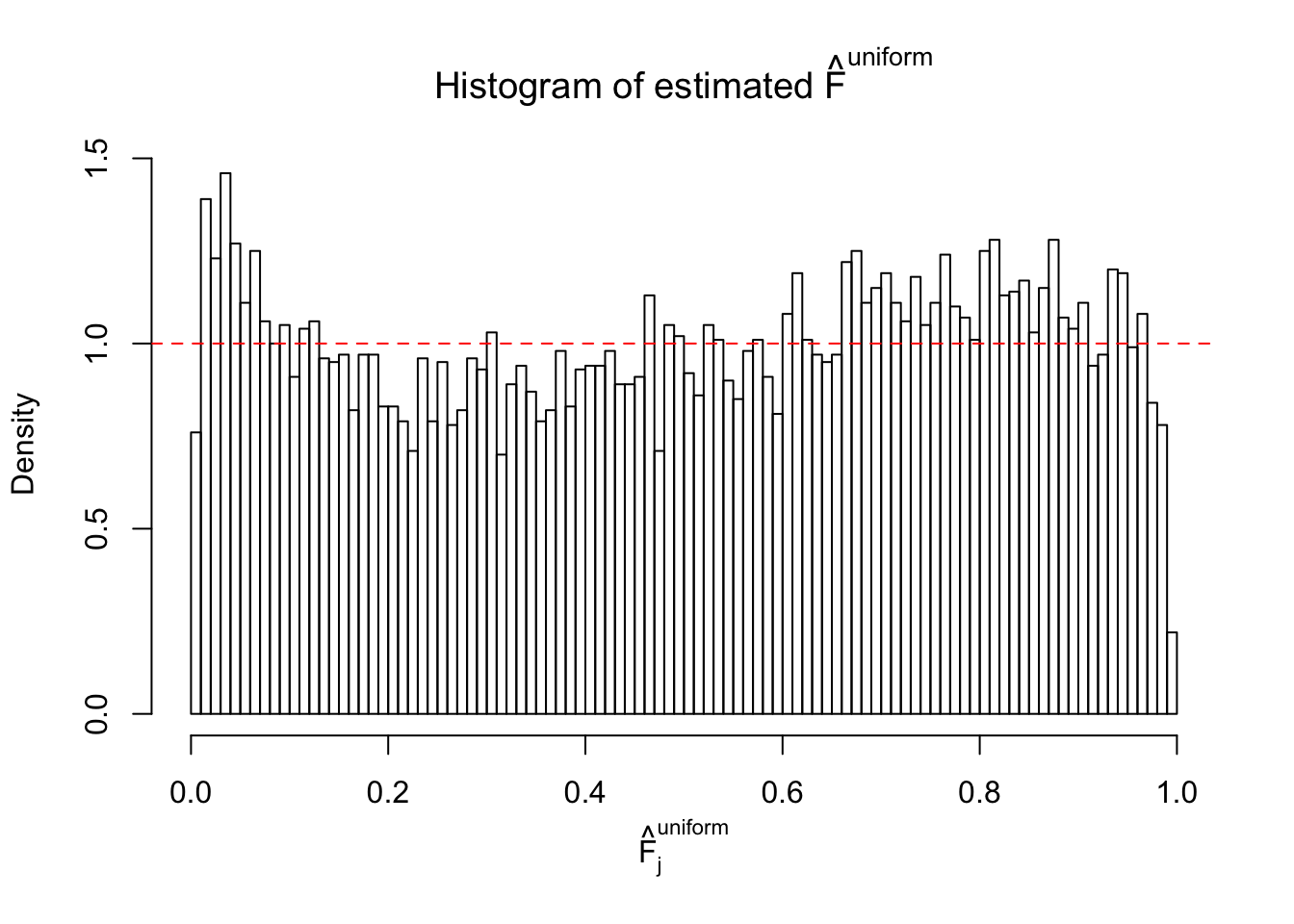
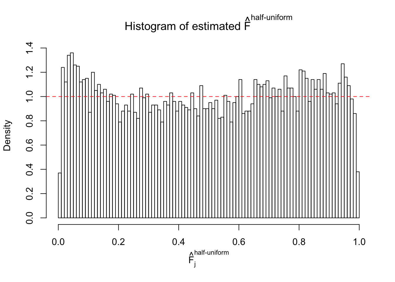
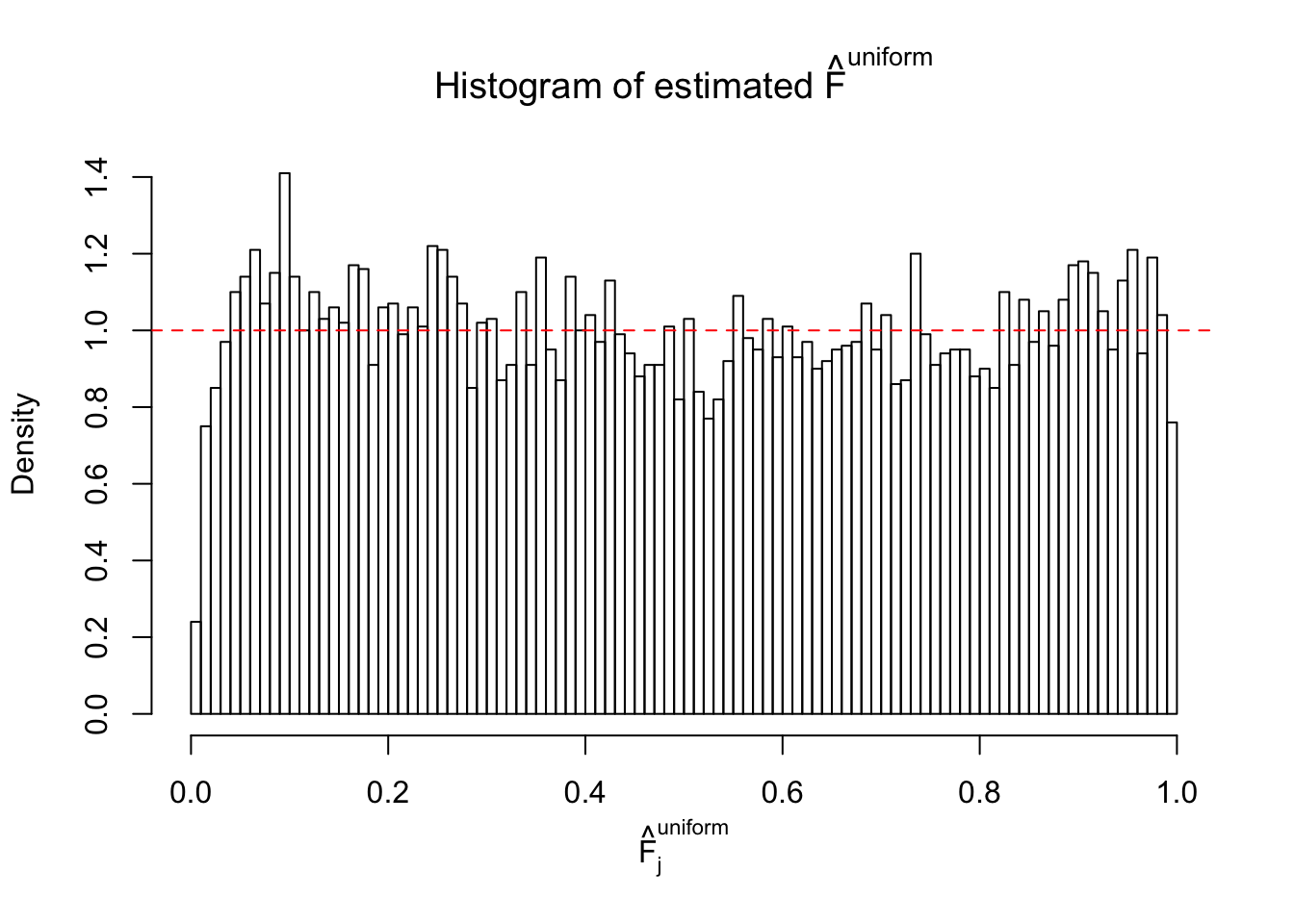
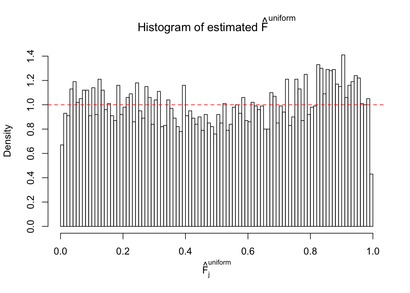
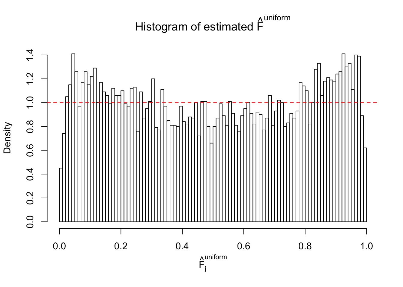
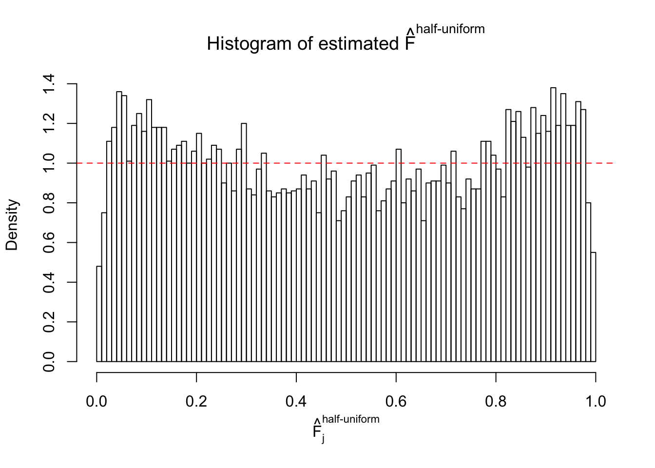
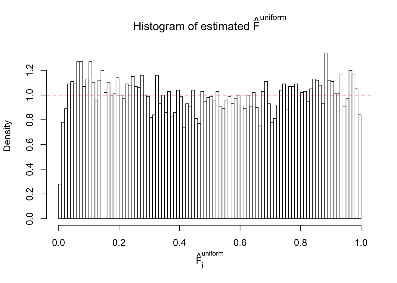
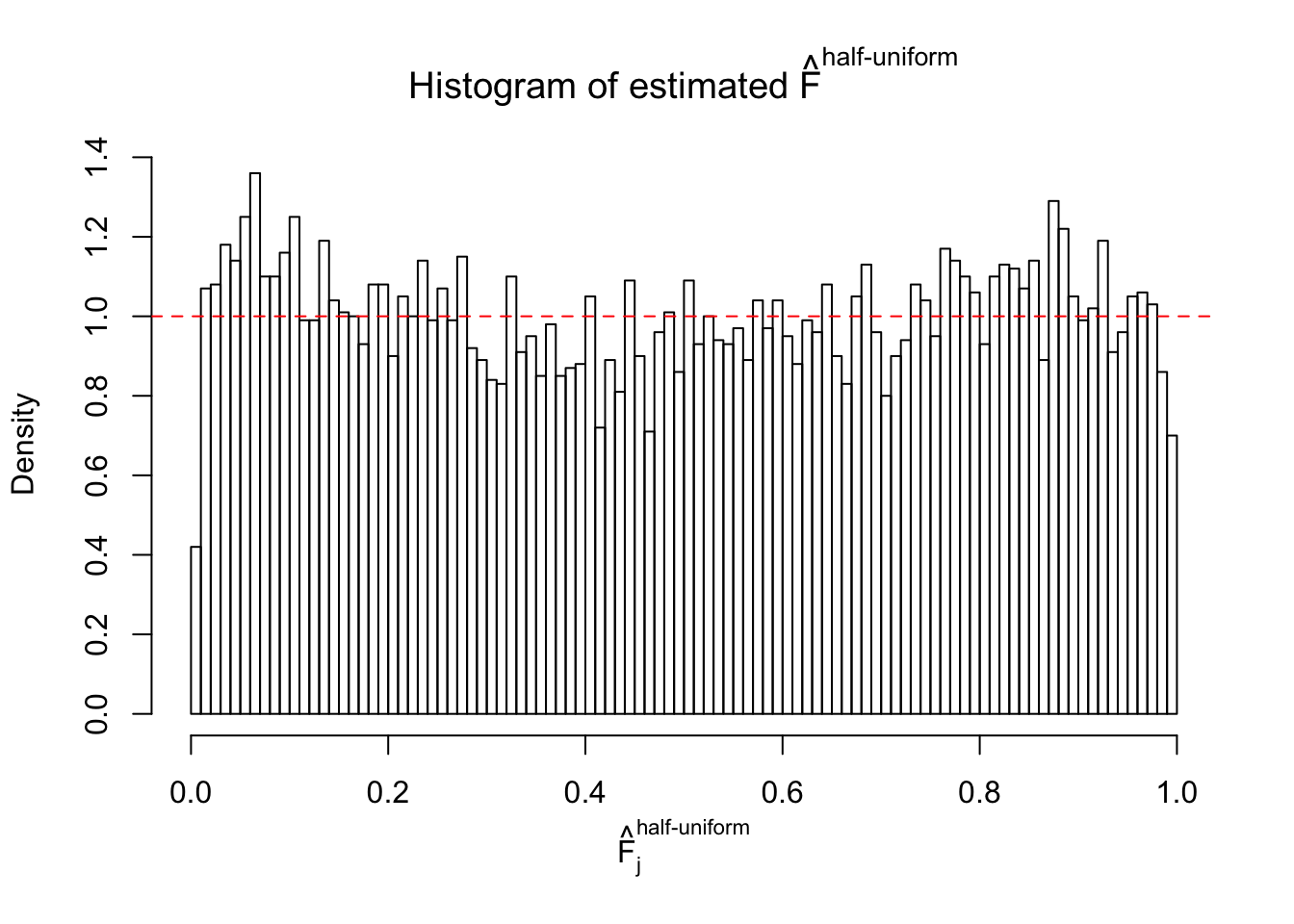
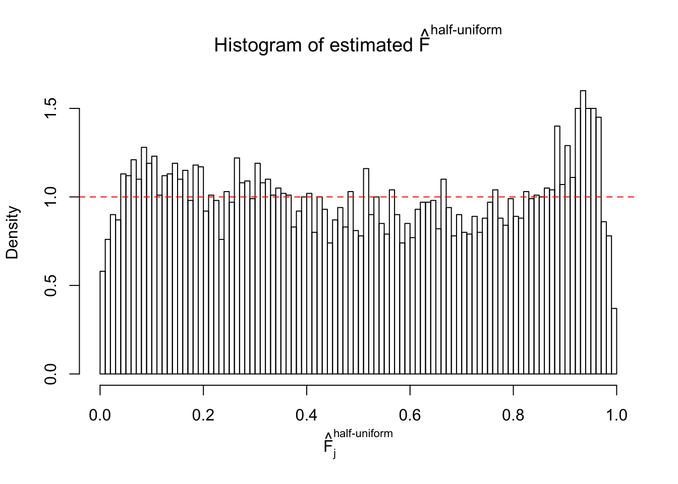
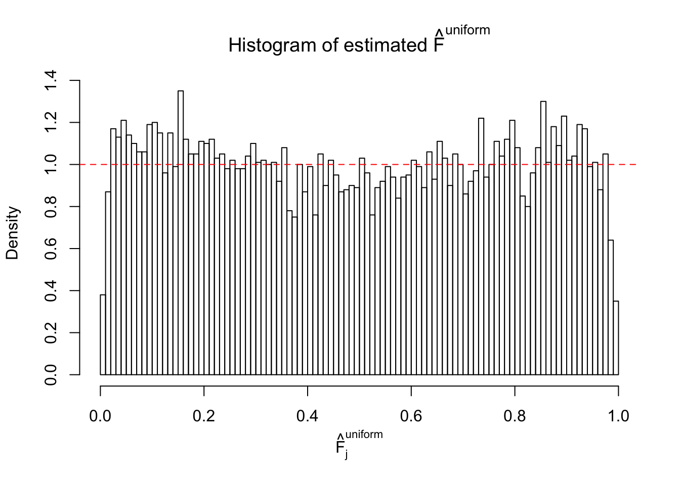
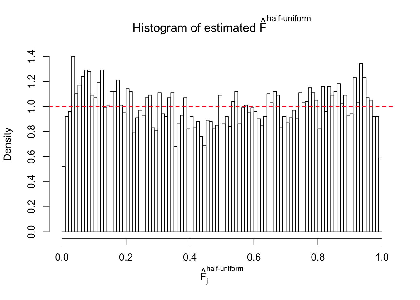
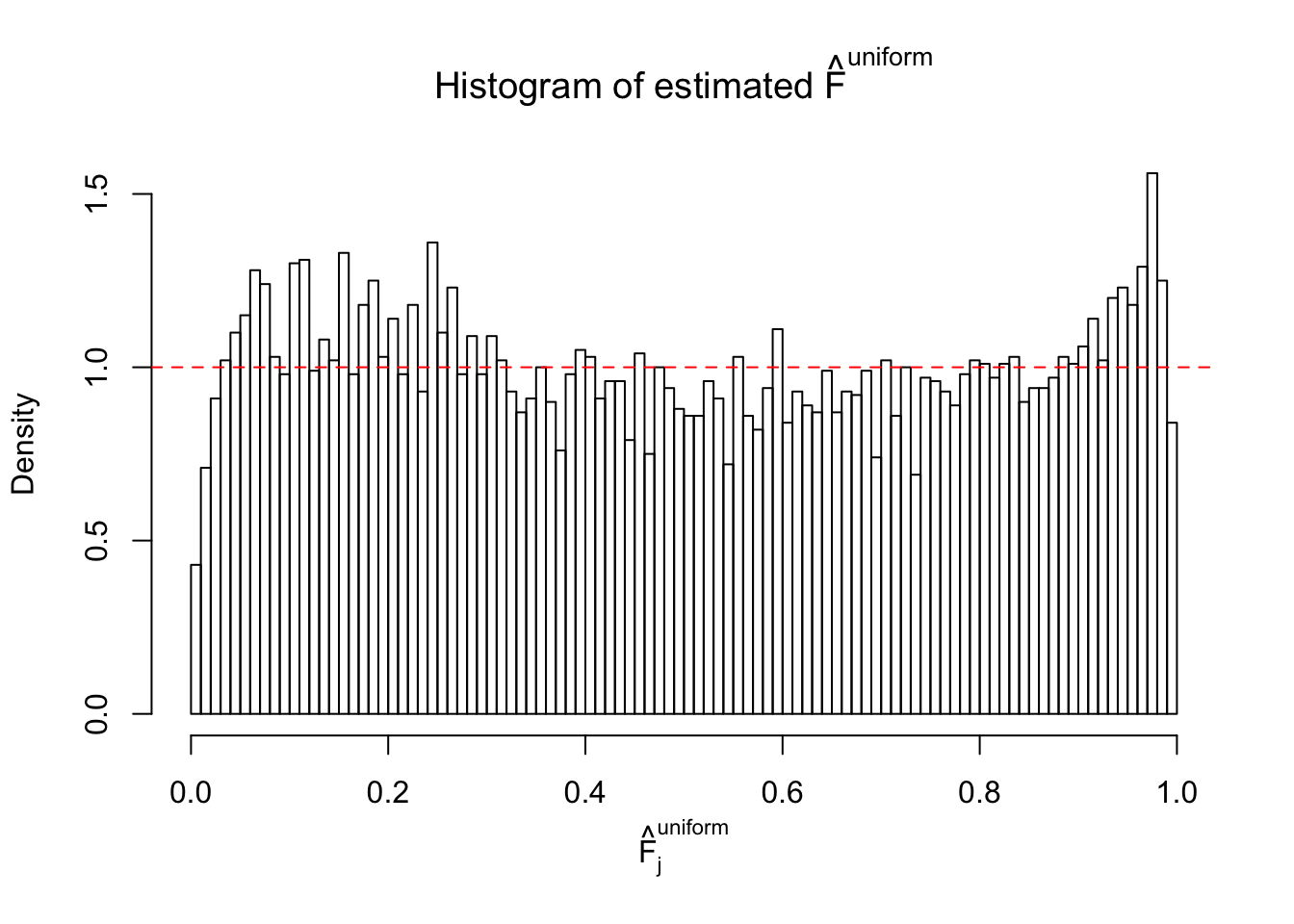
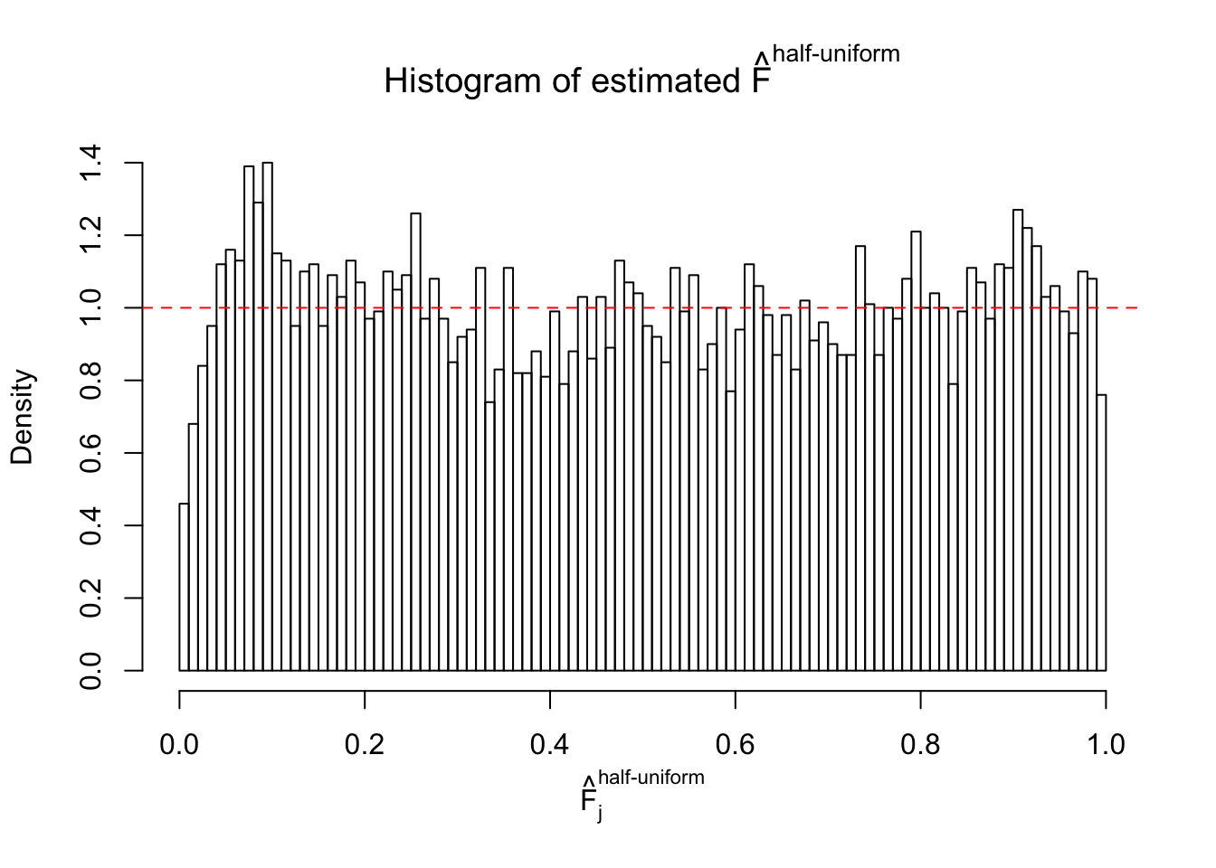
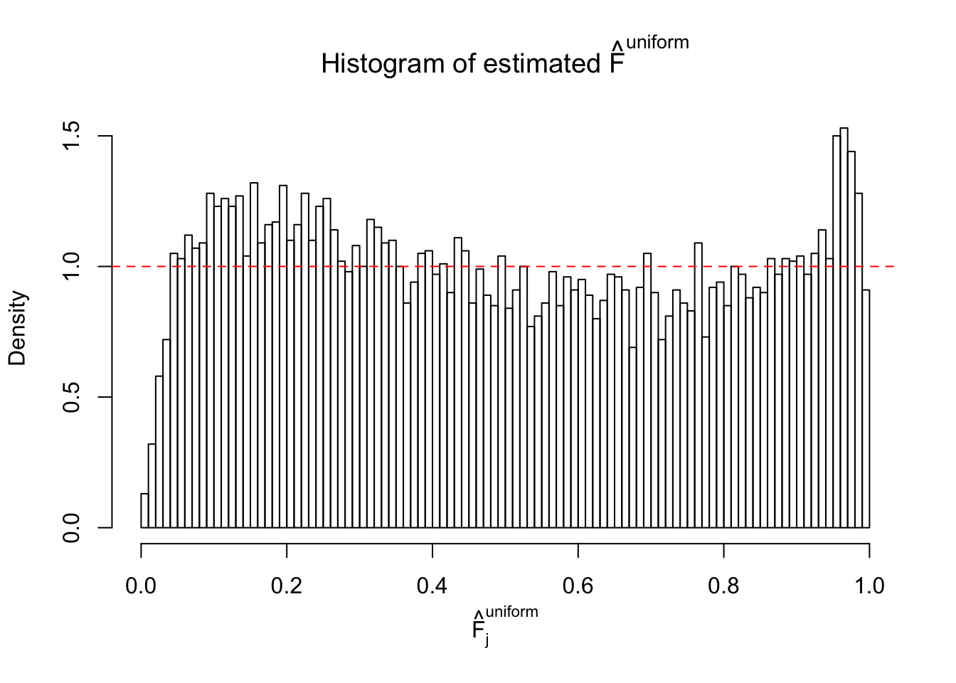
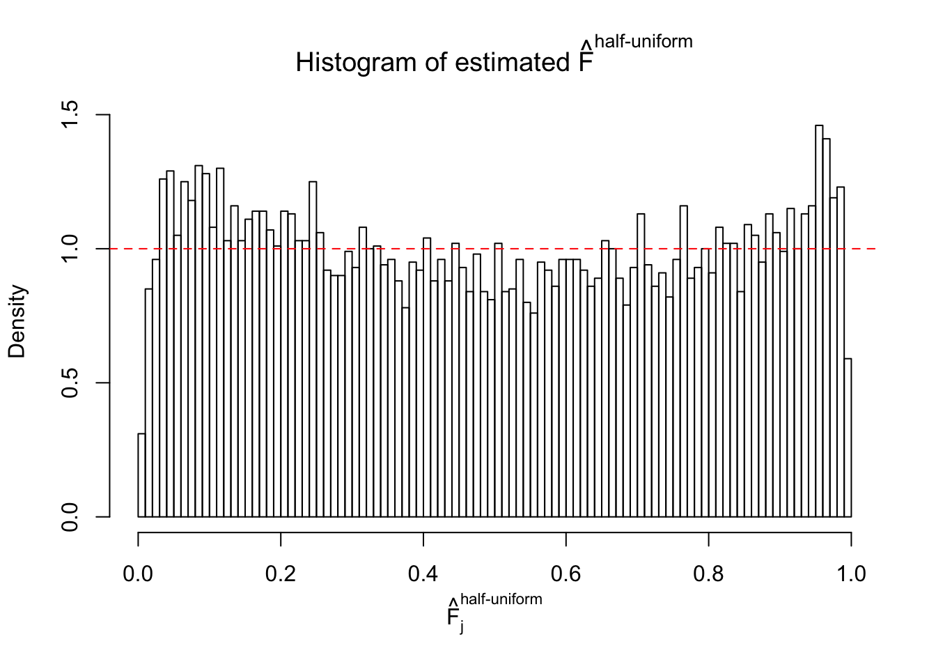
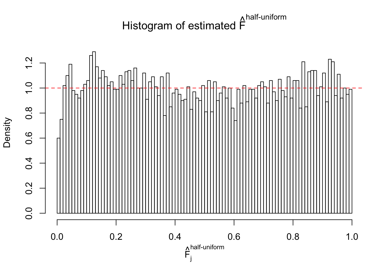
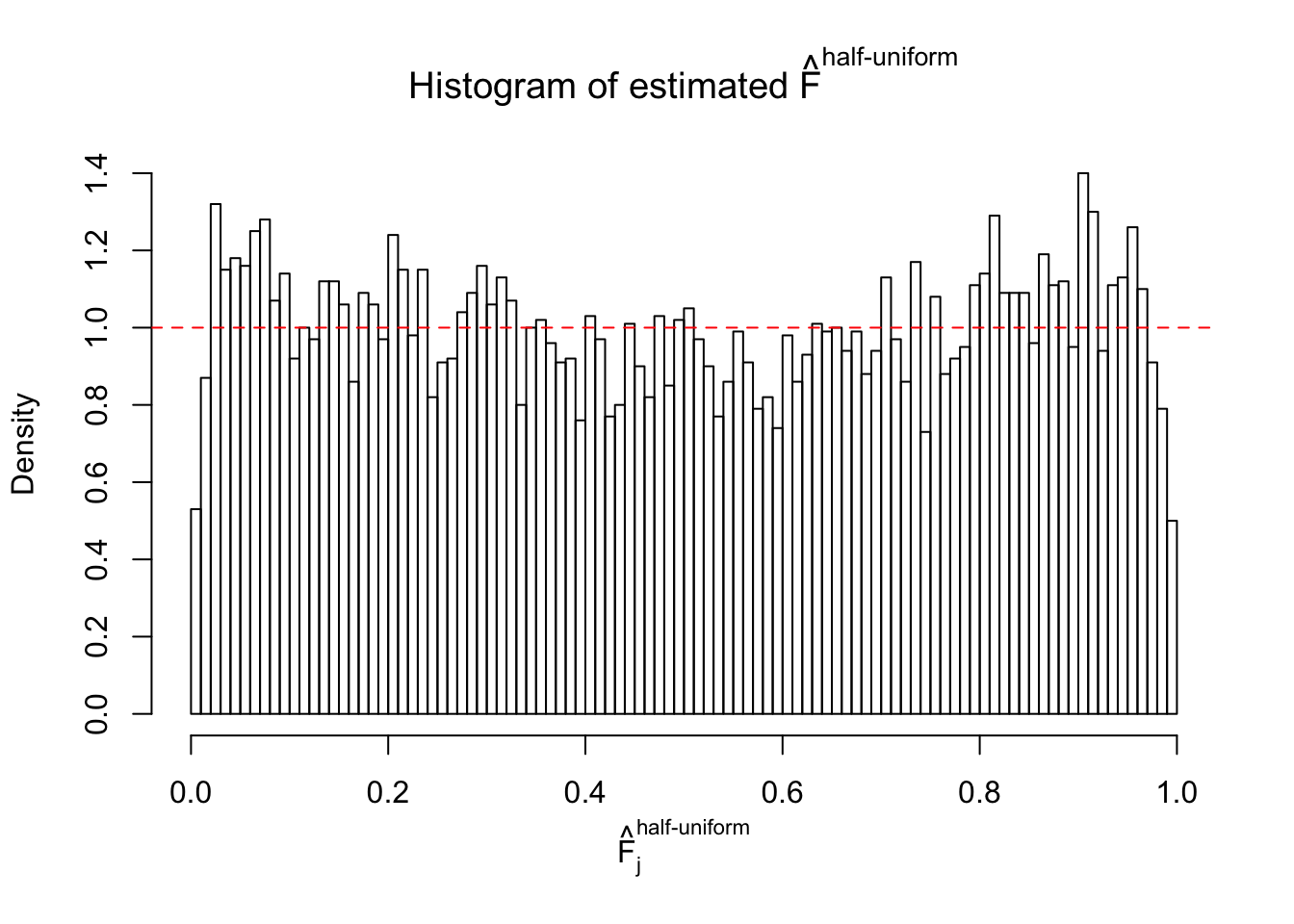
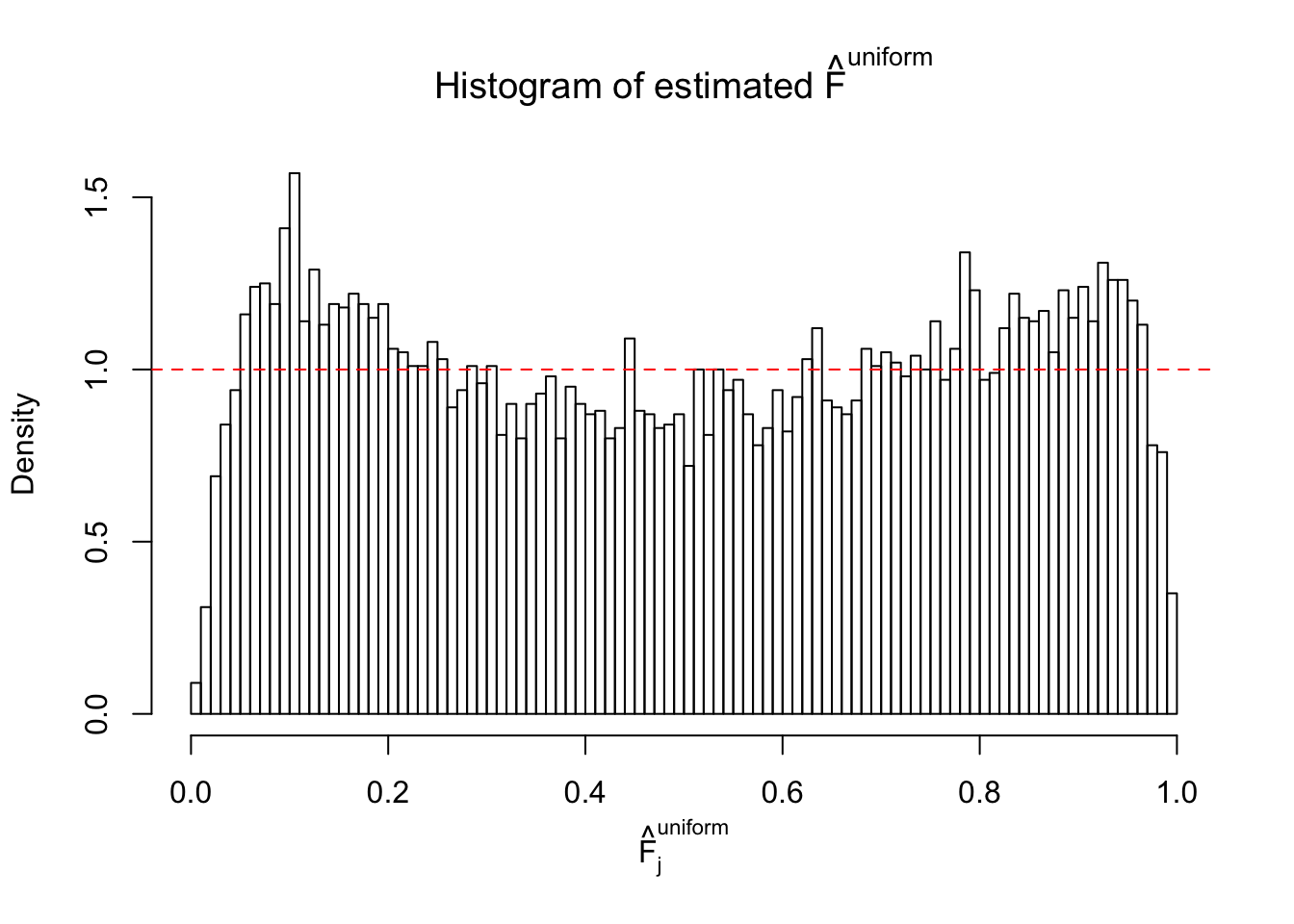
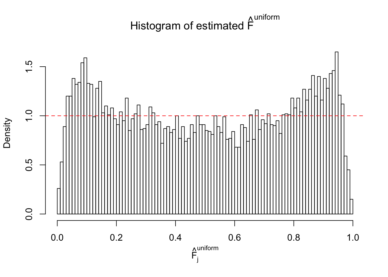
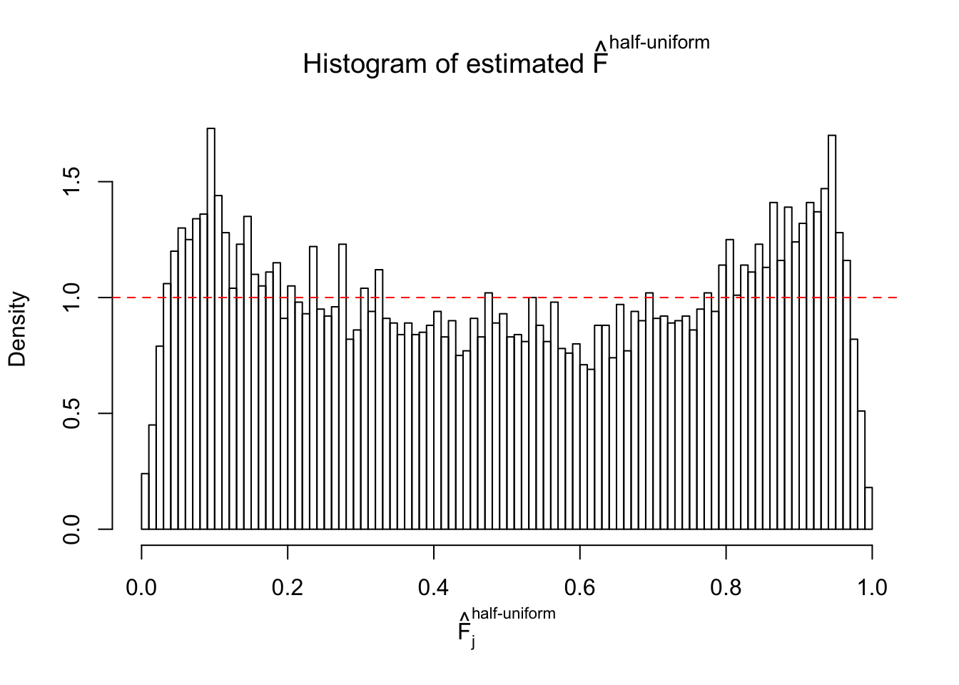
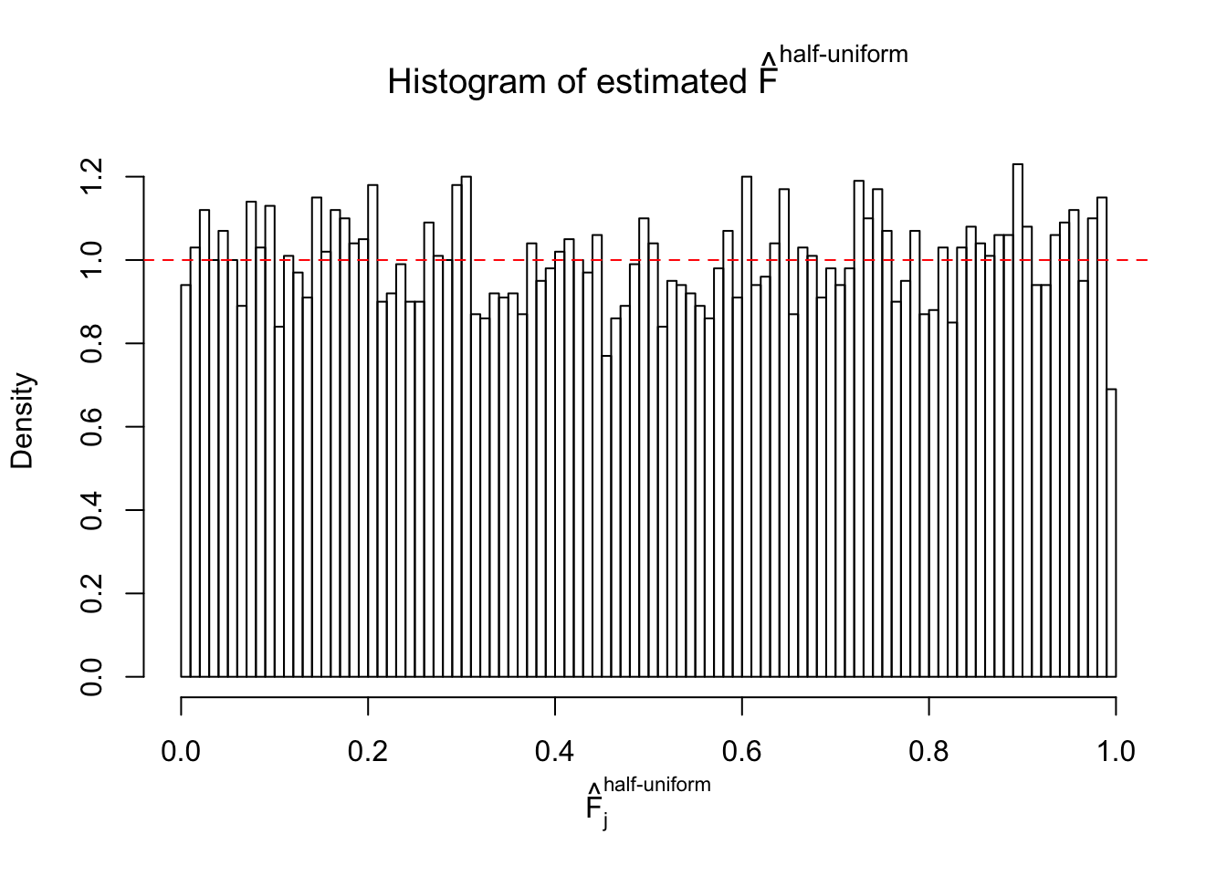
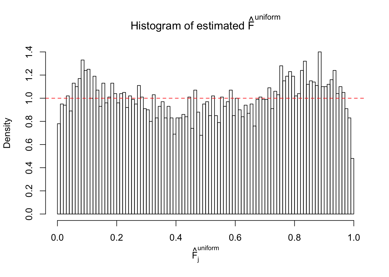
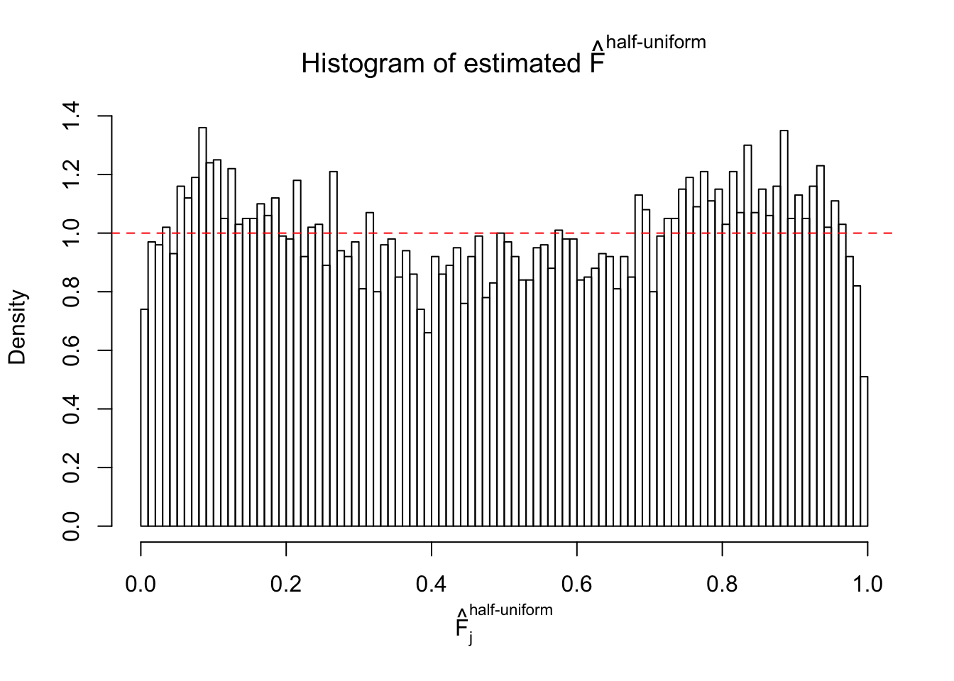
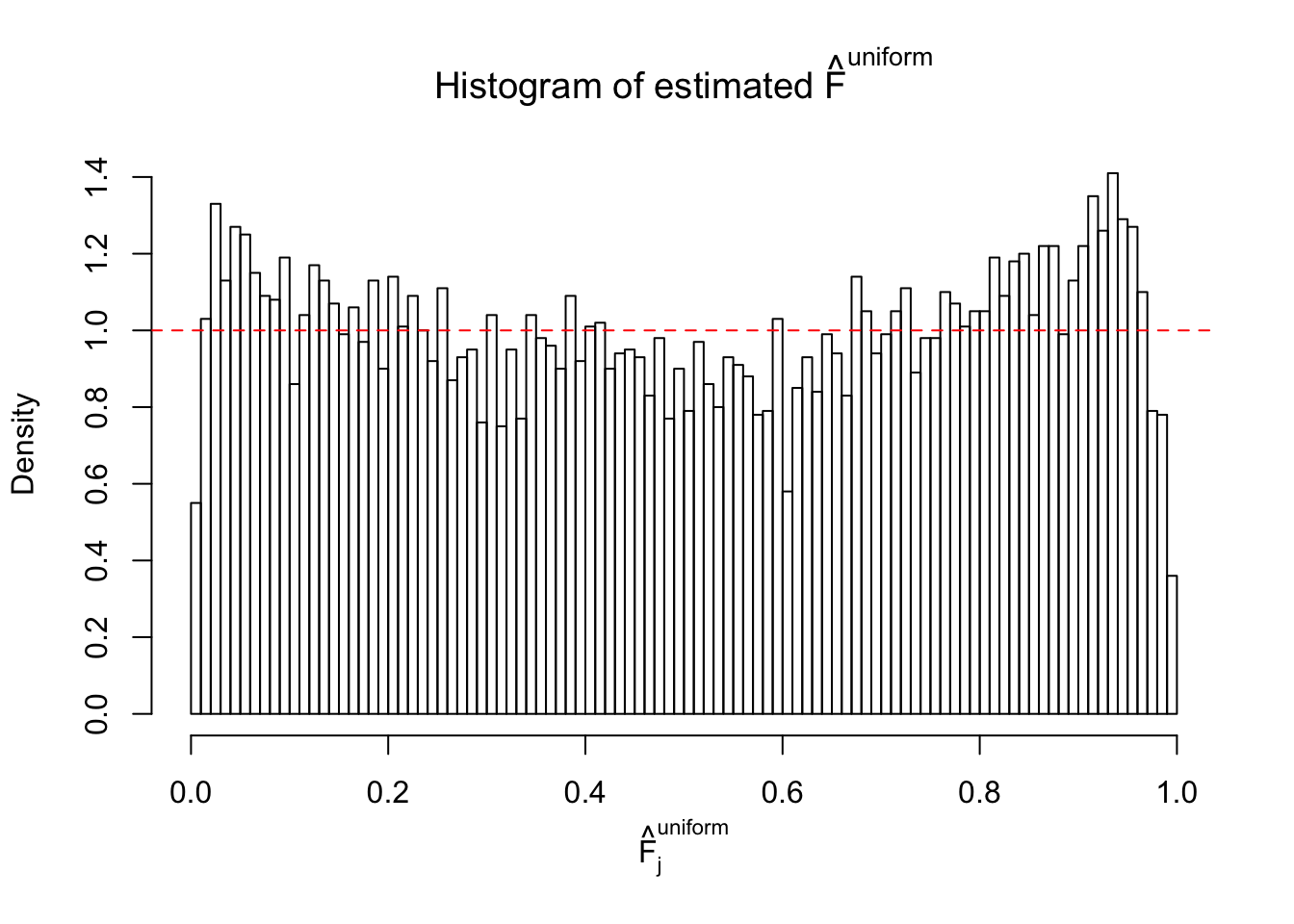
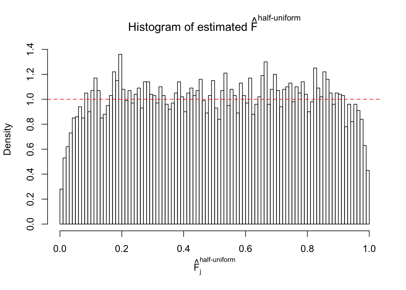
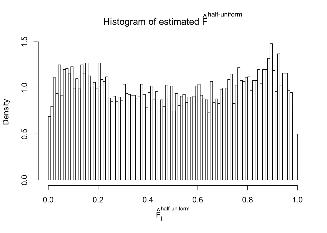
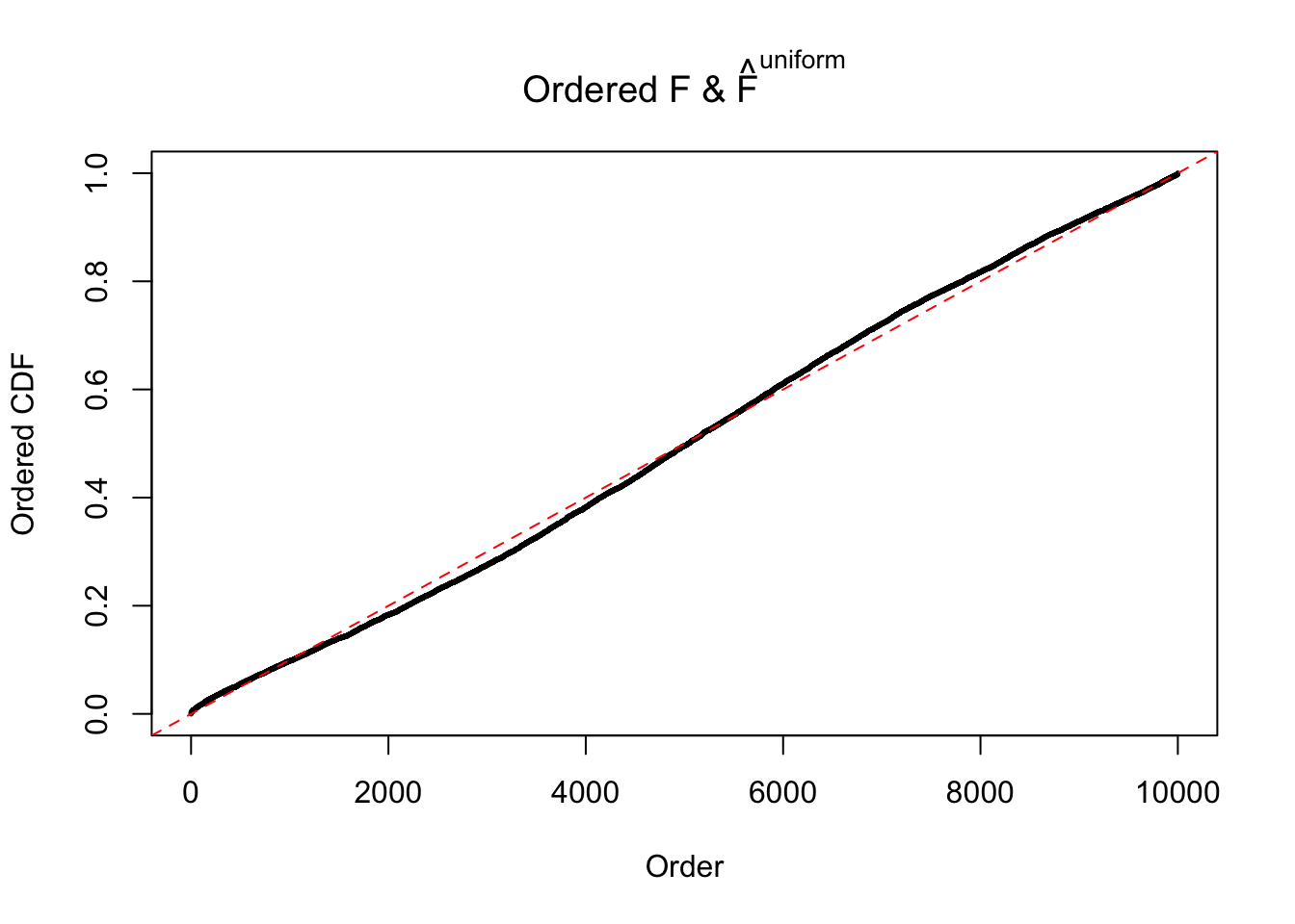
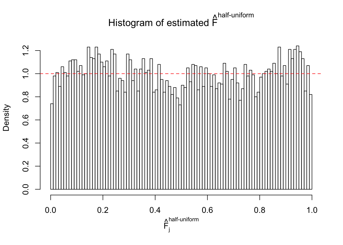
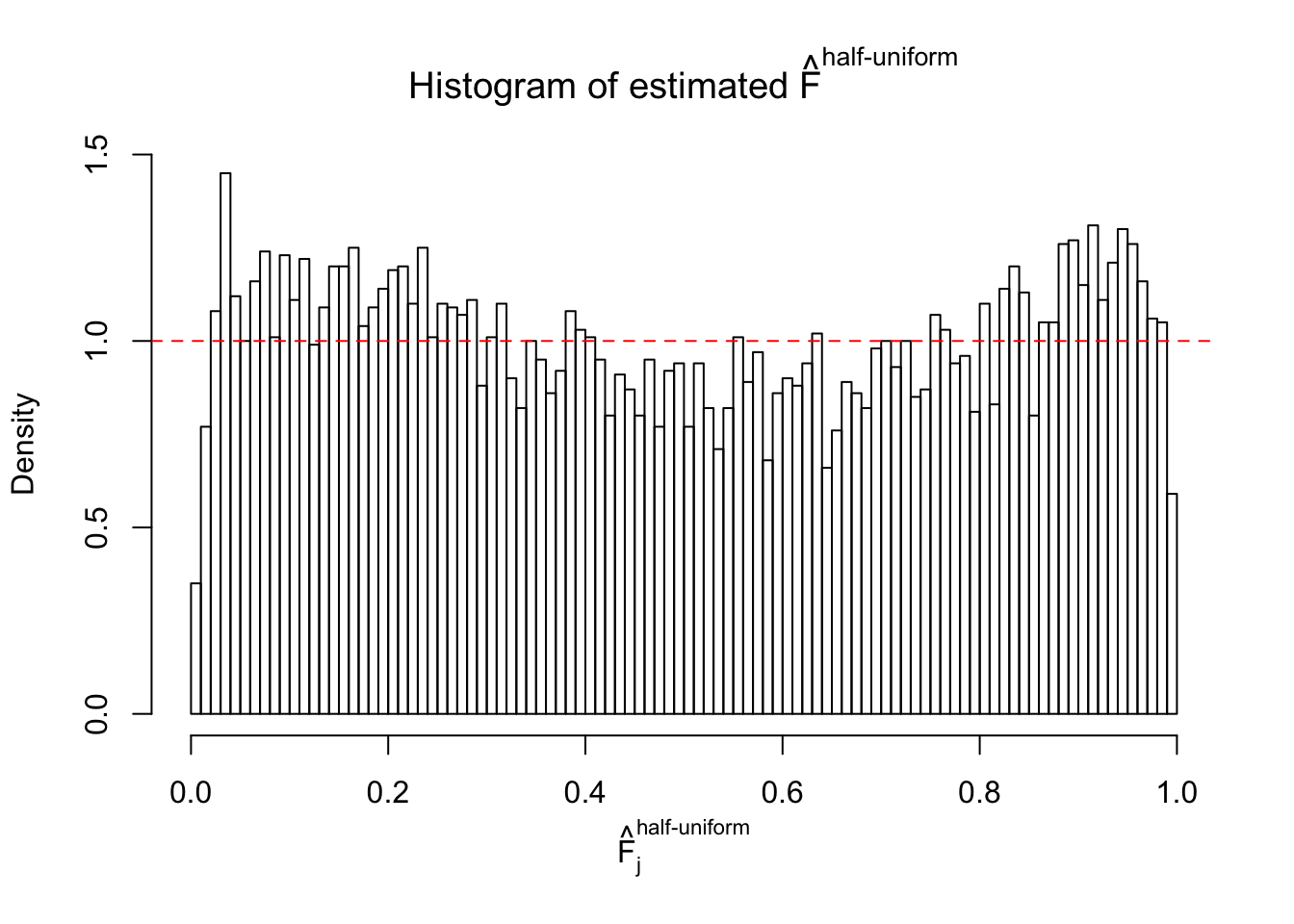
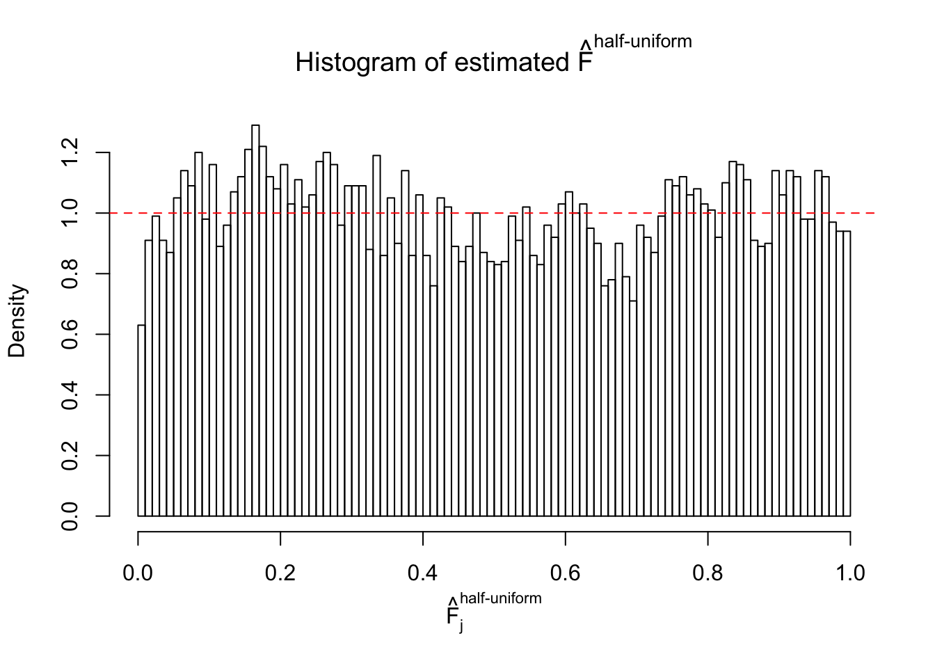
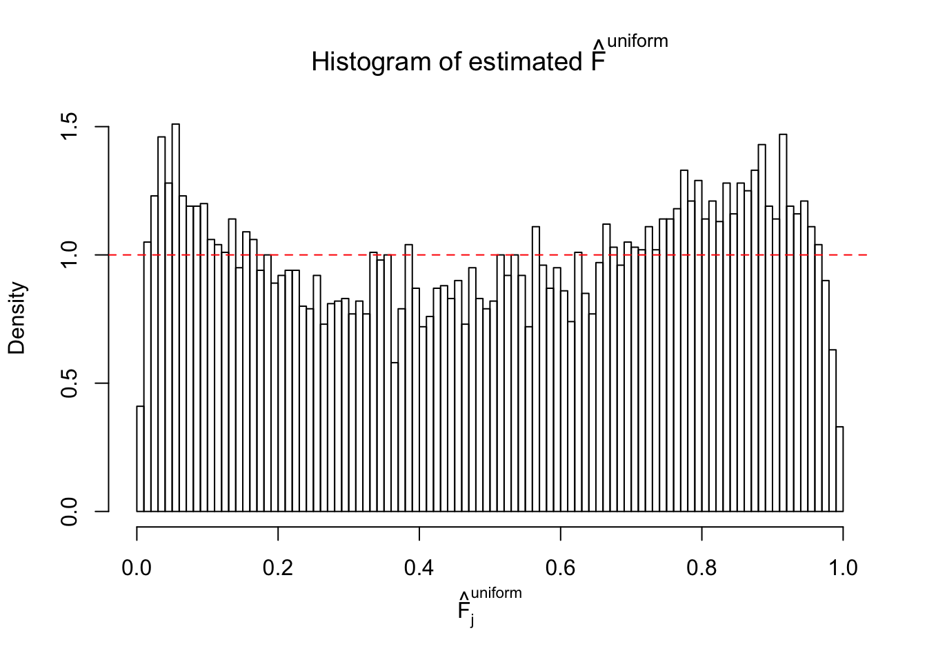
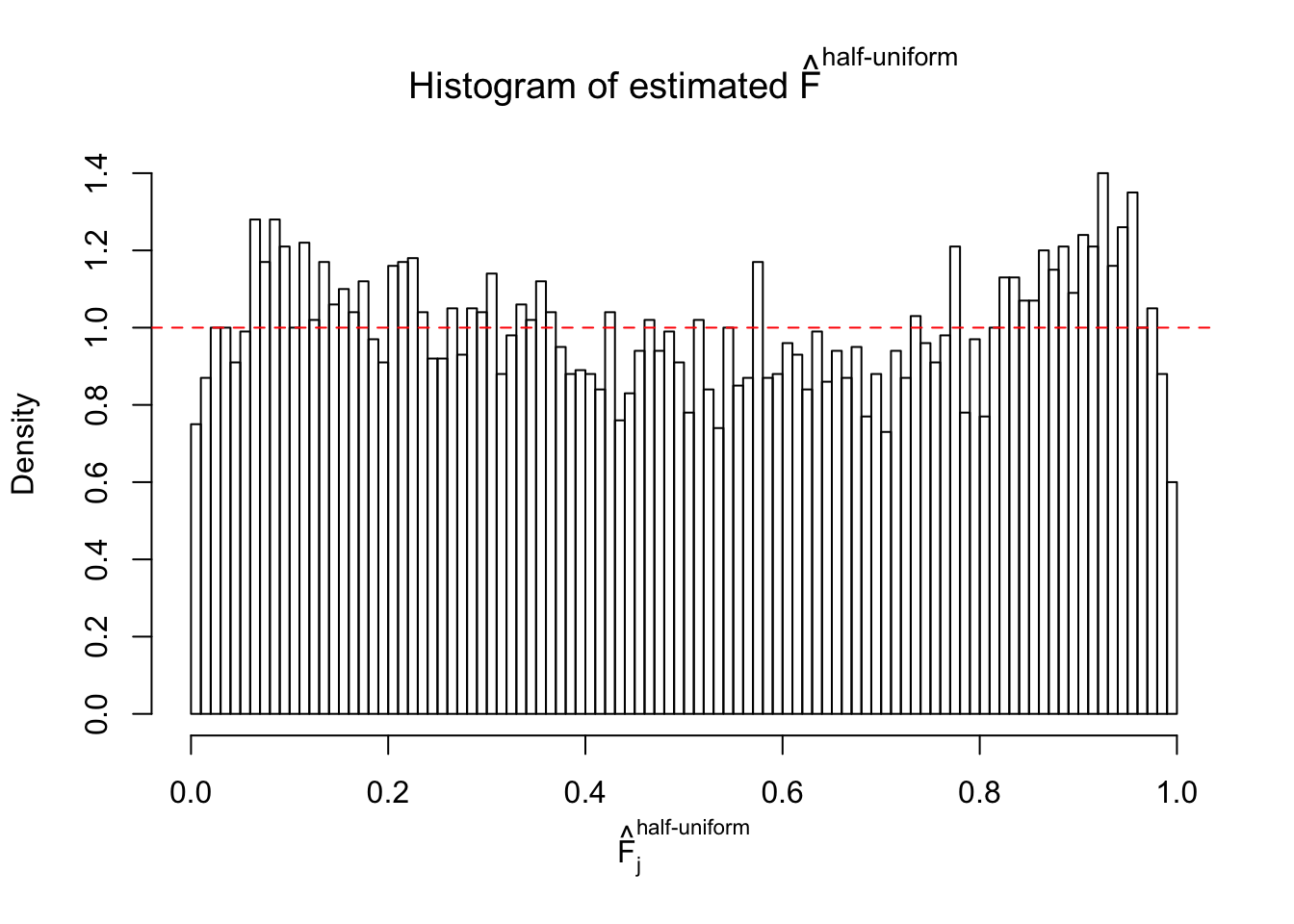
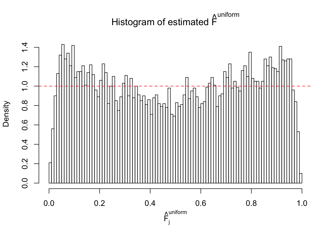
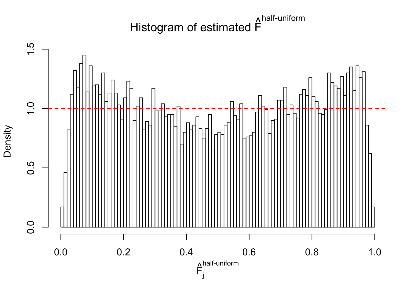
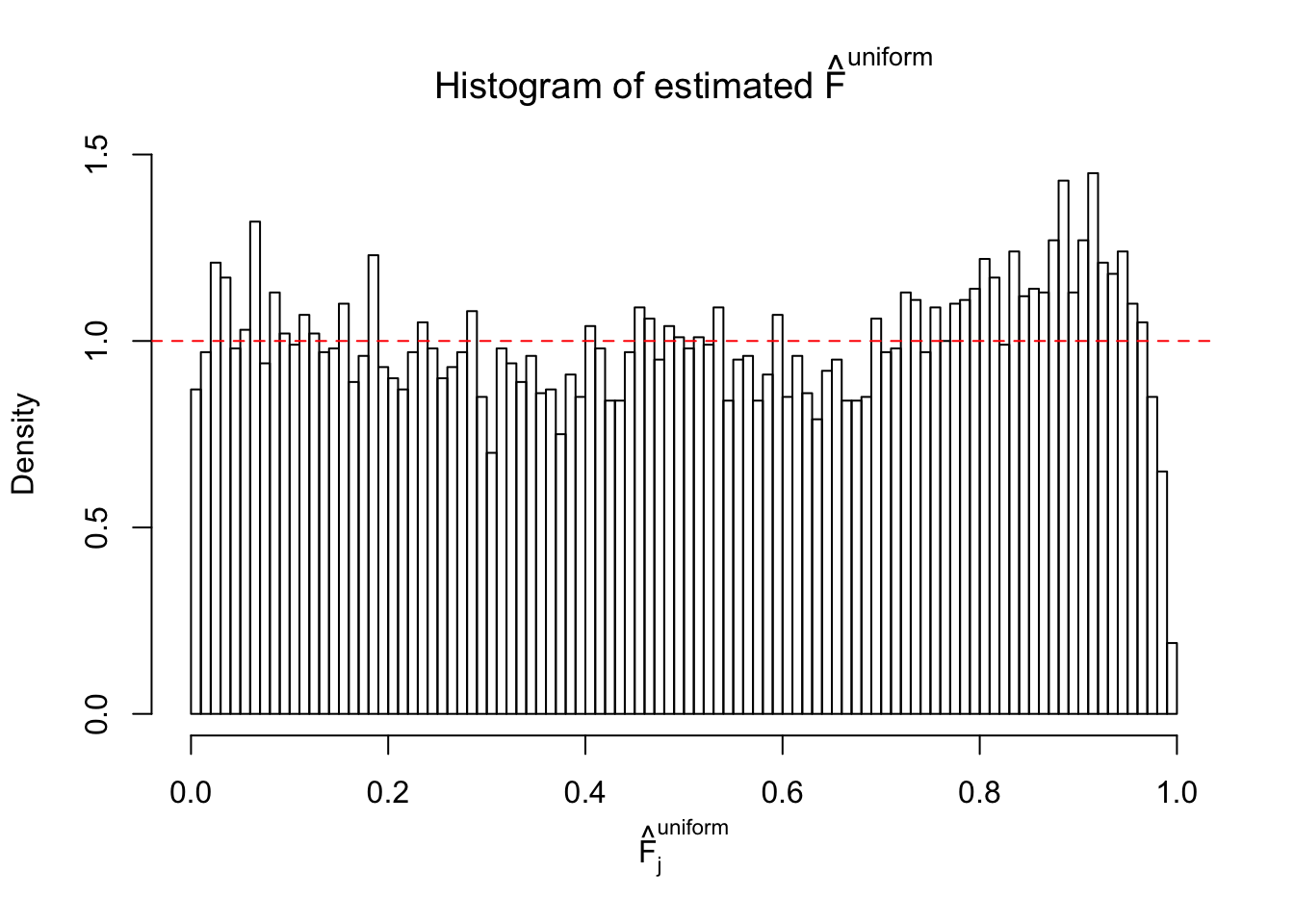
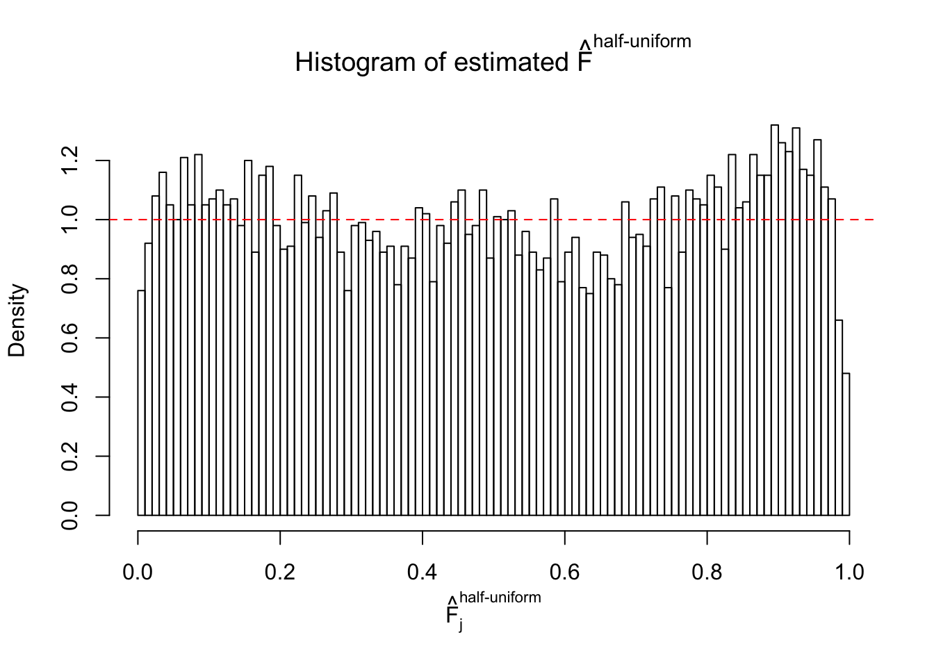
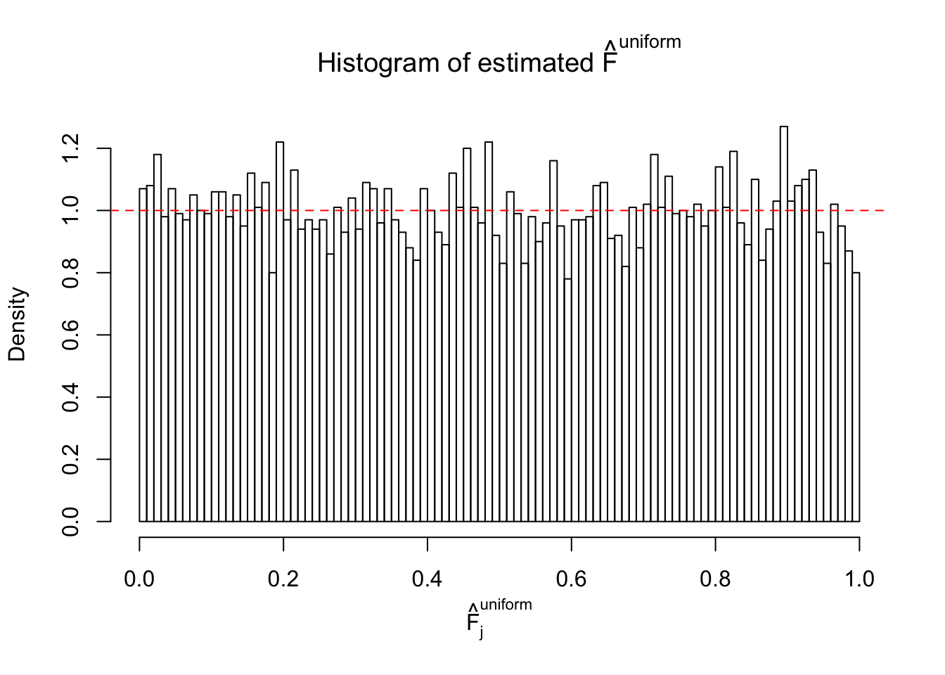
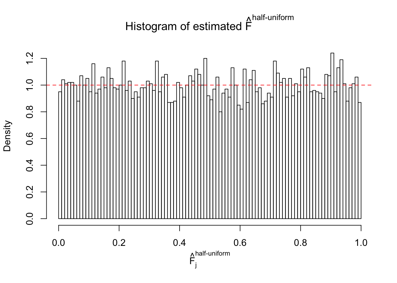
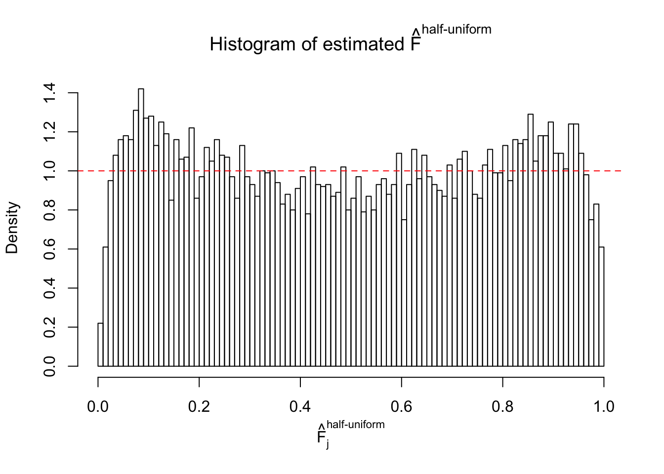
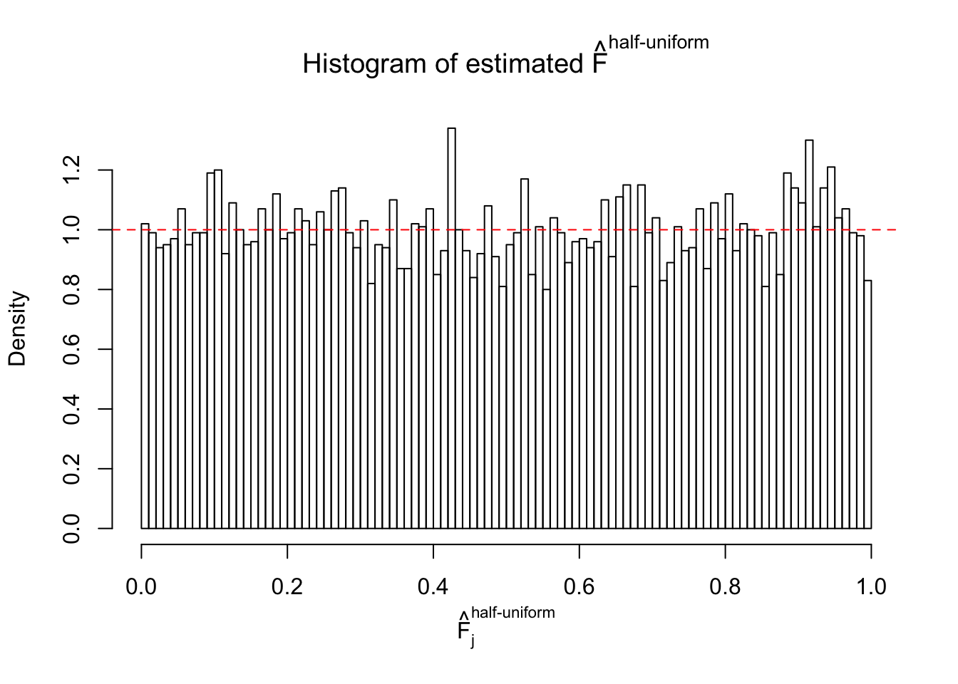
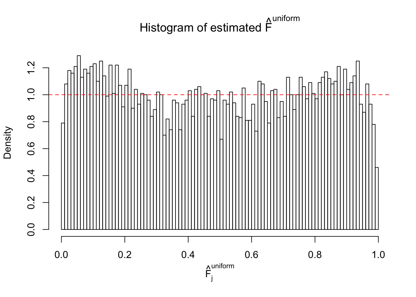
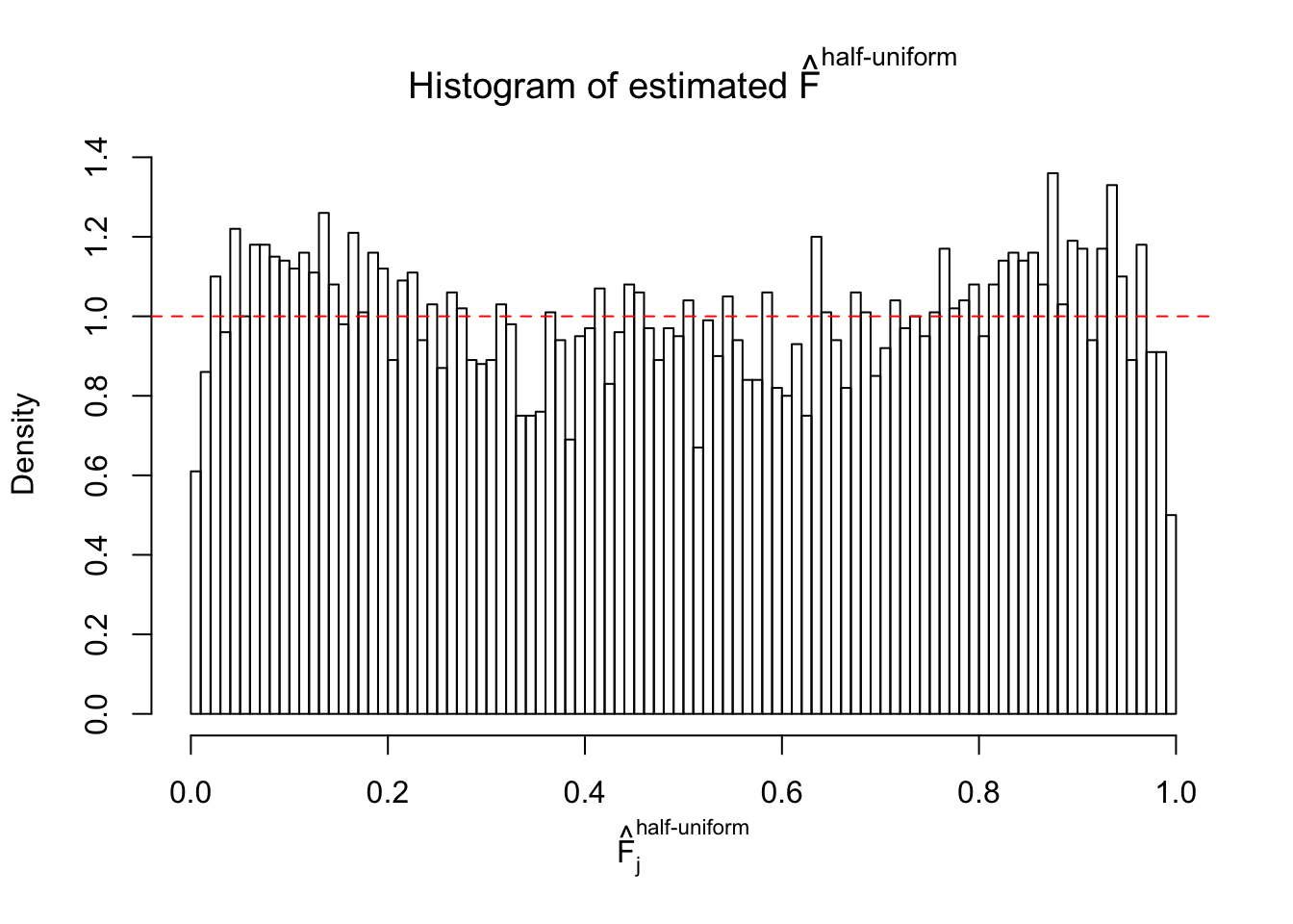
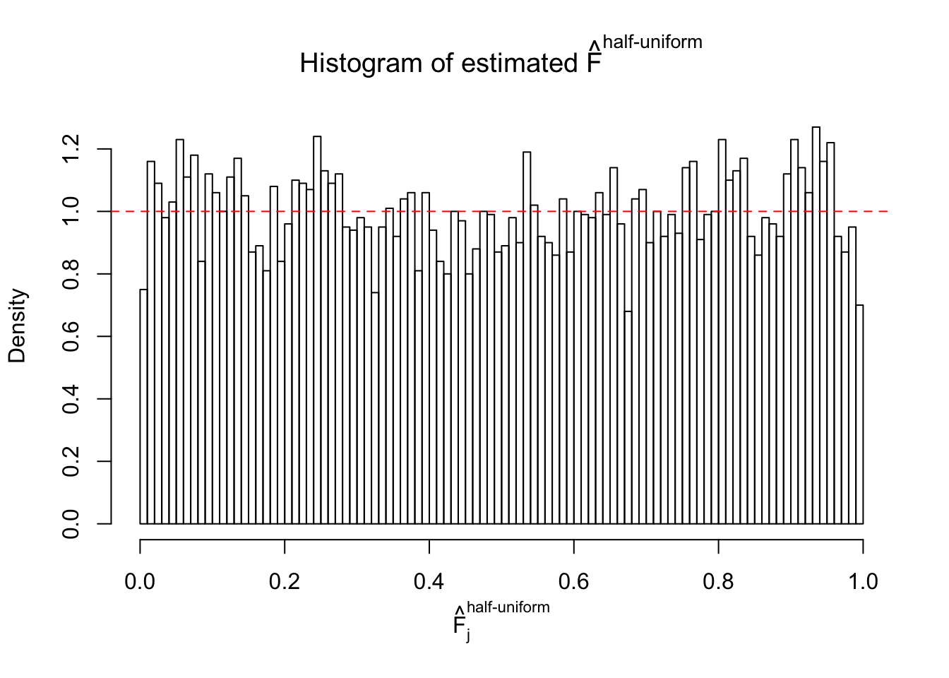
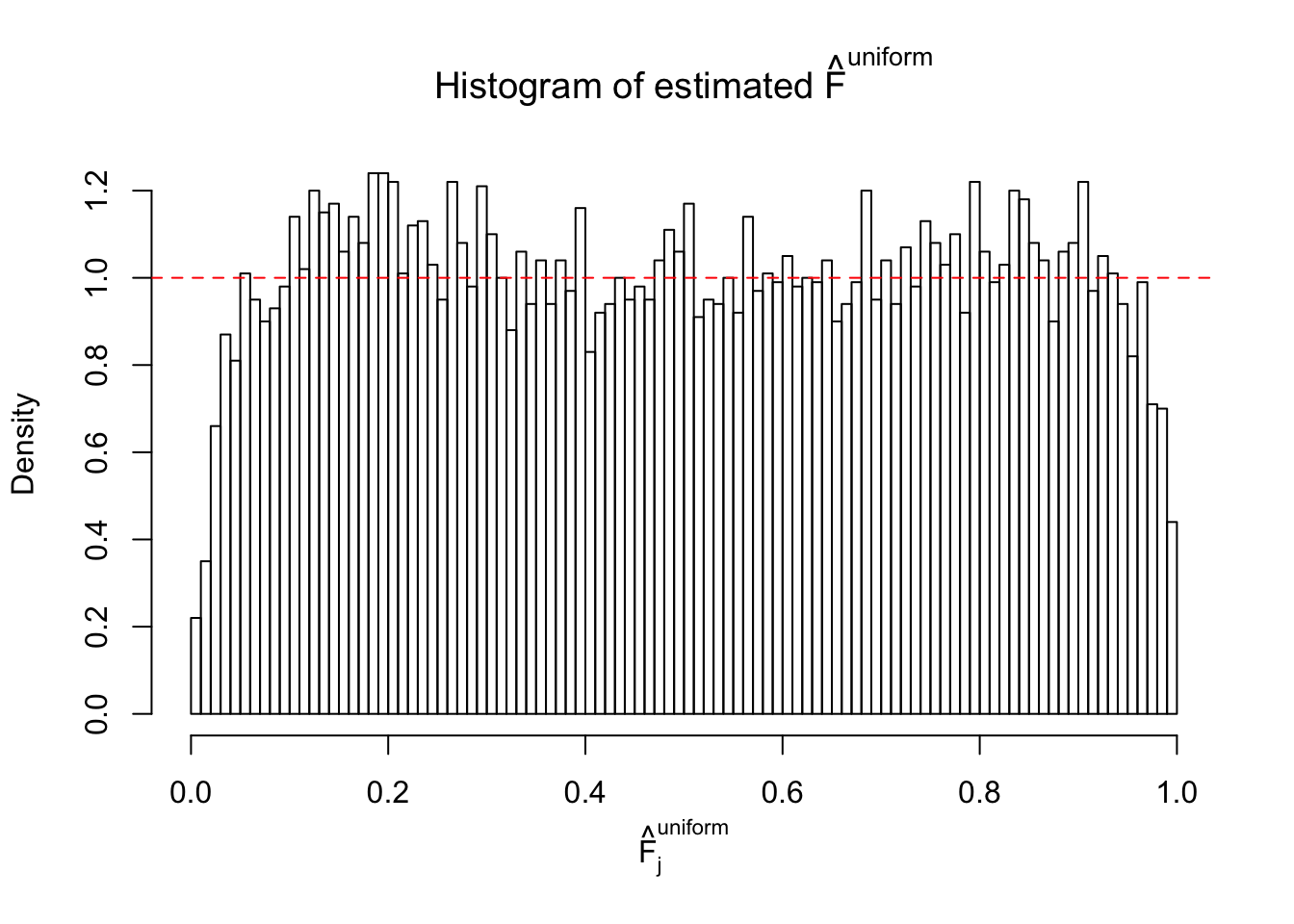
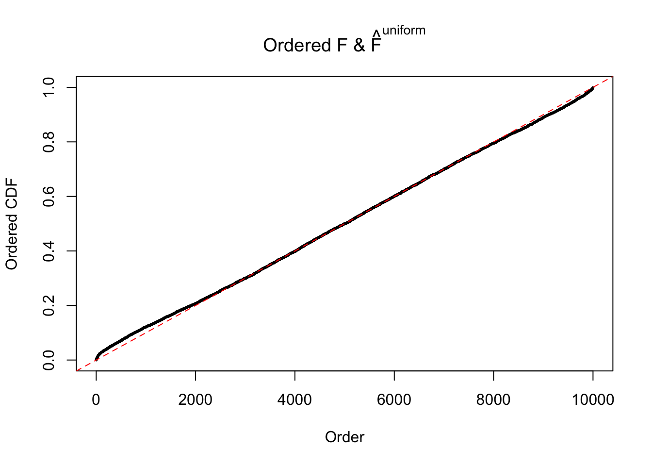
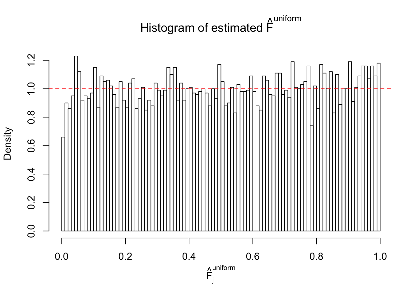
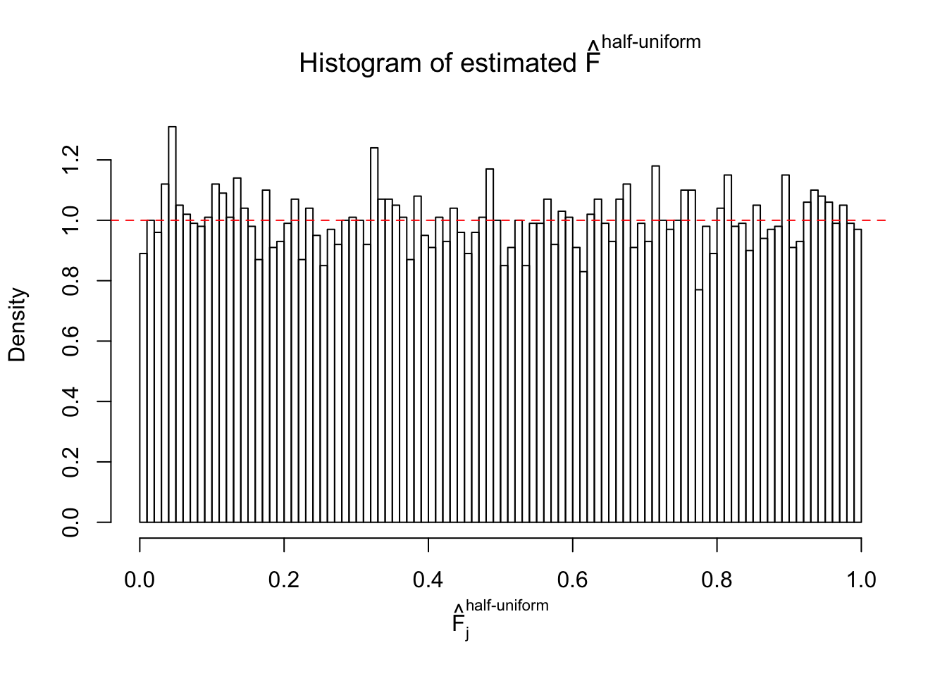
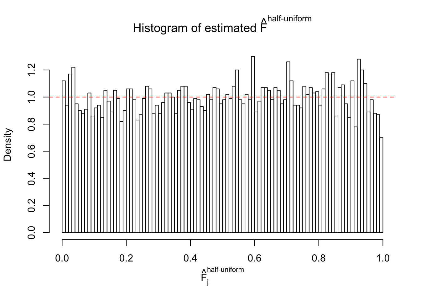
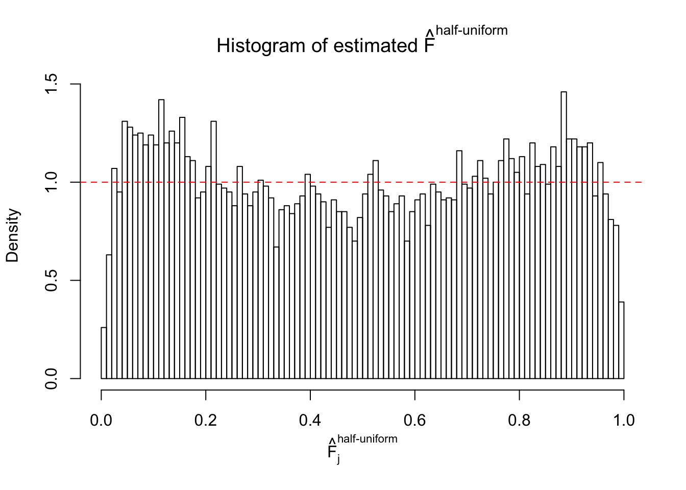
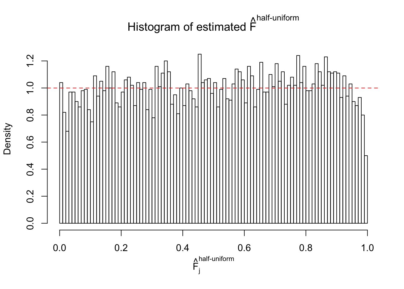
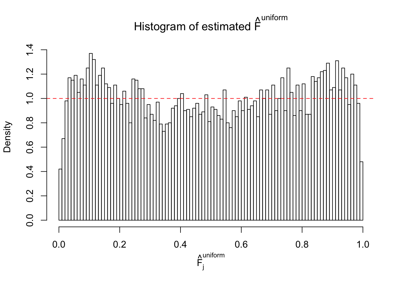
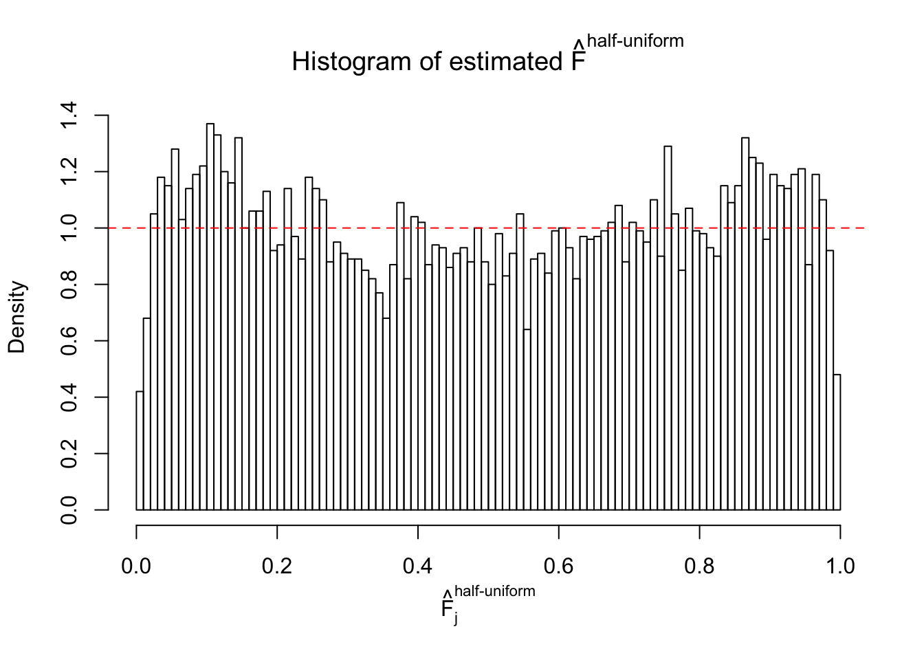
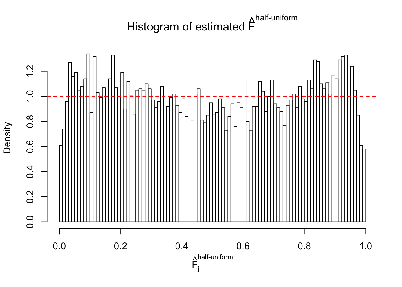
m = ncol(z)It’s worth noting that for the same data set, that is, for the same correlated \(z\) scores, the diagnostic plots of ASH using a mixture uniform prior is usually conspicuously better than those using a mixture normal prior. This might be because uniform mixtures are more flexible than normal mixtures at dealing with irregular distributions, like the “moderates inflated yet extremes not inflated” one. For the same reason, mixcompdist = "halfuniform" is occasionally better than mixcompdist = "uniform".
N0. 1 : Data Set 355 ; Number of False Discoveries: 639 ; pihat0 = 0.01079742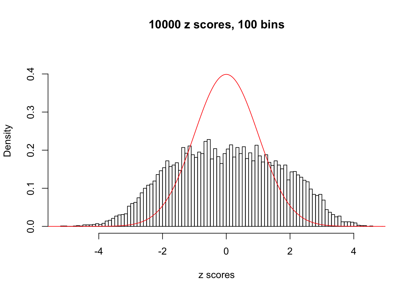


N0. 2 : Data Set 327 ; Number of False Discoveries: 489 ; pihat0 = 0.0477939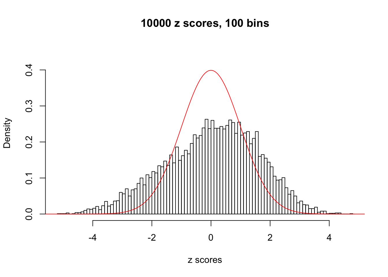


N0. 3 : Data Set 23 ; Number of False Discoveries: 408 ; pihat0 = 0.008419777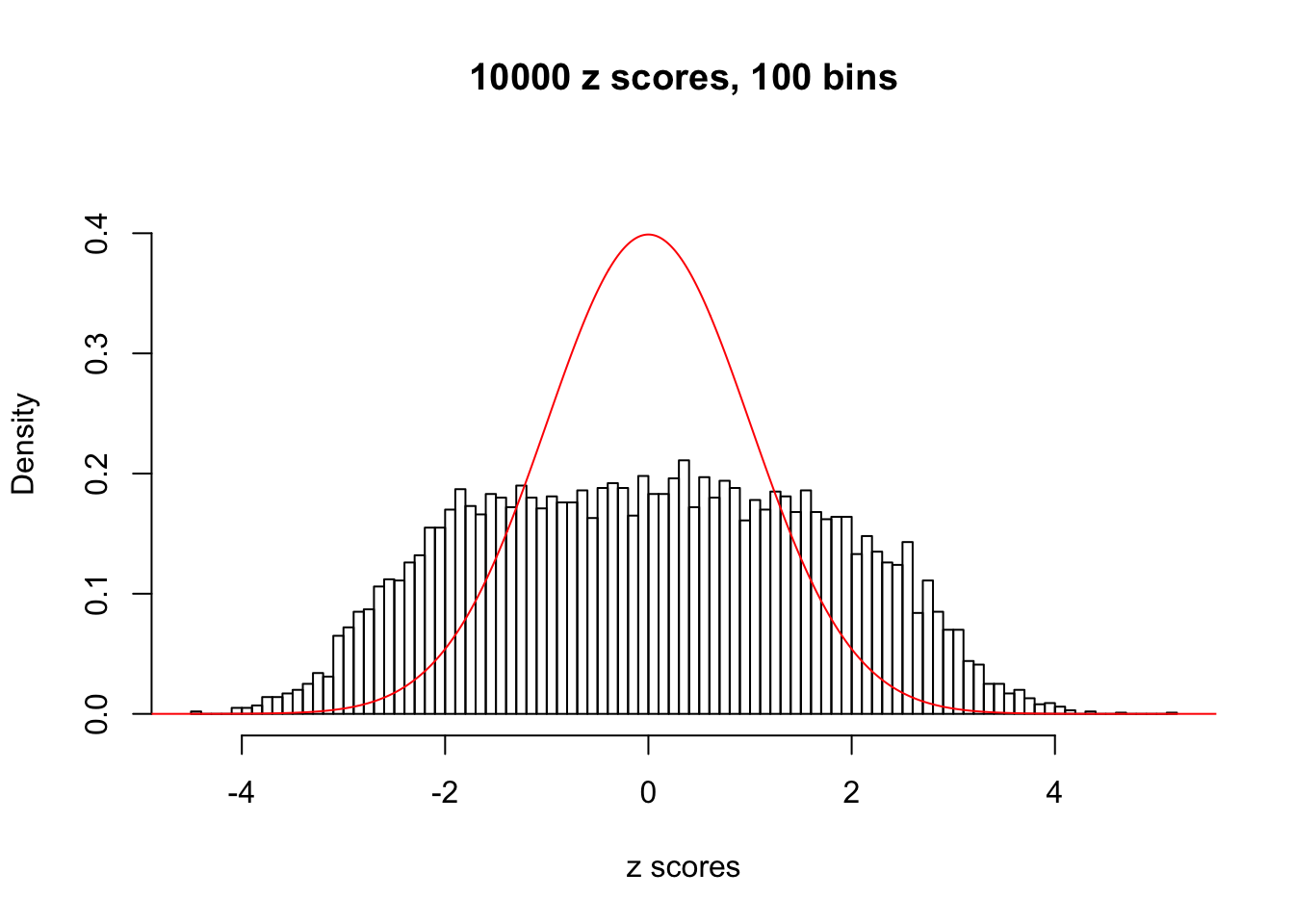


N0. 4 : Data Set 122 ; Number of False Discoveries: 331 ; pihat0 = 0.01544099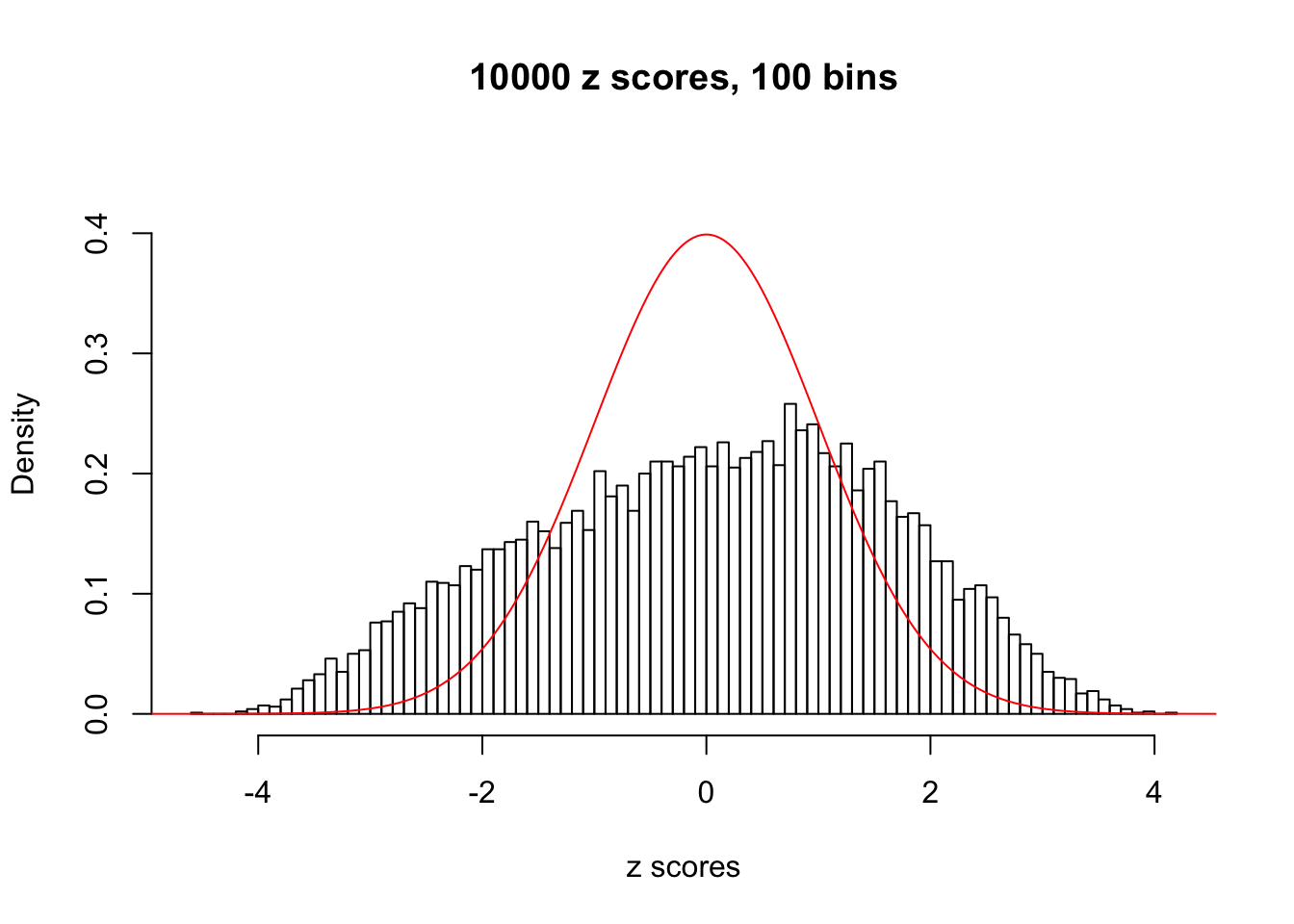


N0. 5 : Data Set 783 ; Number of False Discoveries: 170 ; pihat0 = 0.01516697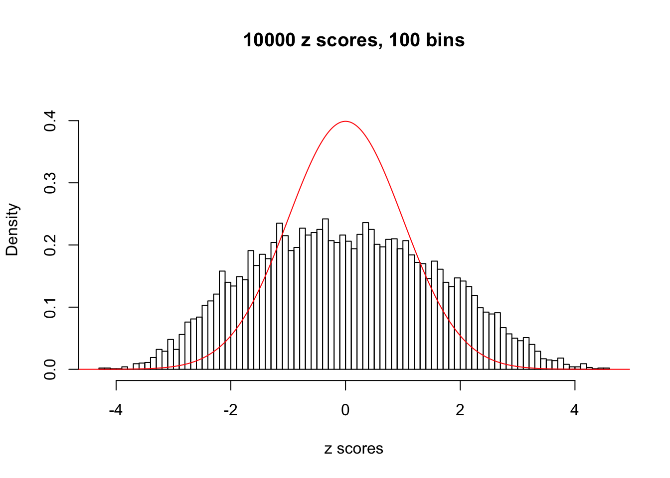


N0. 6 : Data Set 749 ; Number of False Discoveries: 114 ; pihat0 = 0.01482747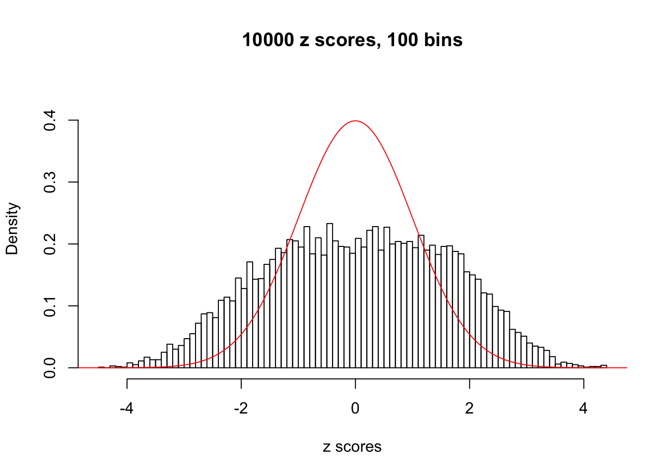


N0. 7 : Data Set 724 ; Number of False Discoveries: 79 ; pihat0 = 0.01451062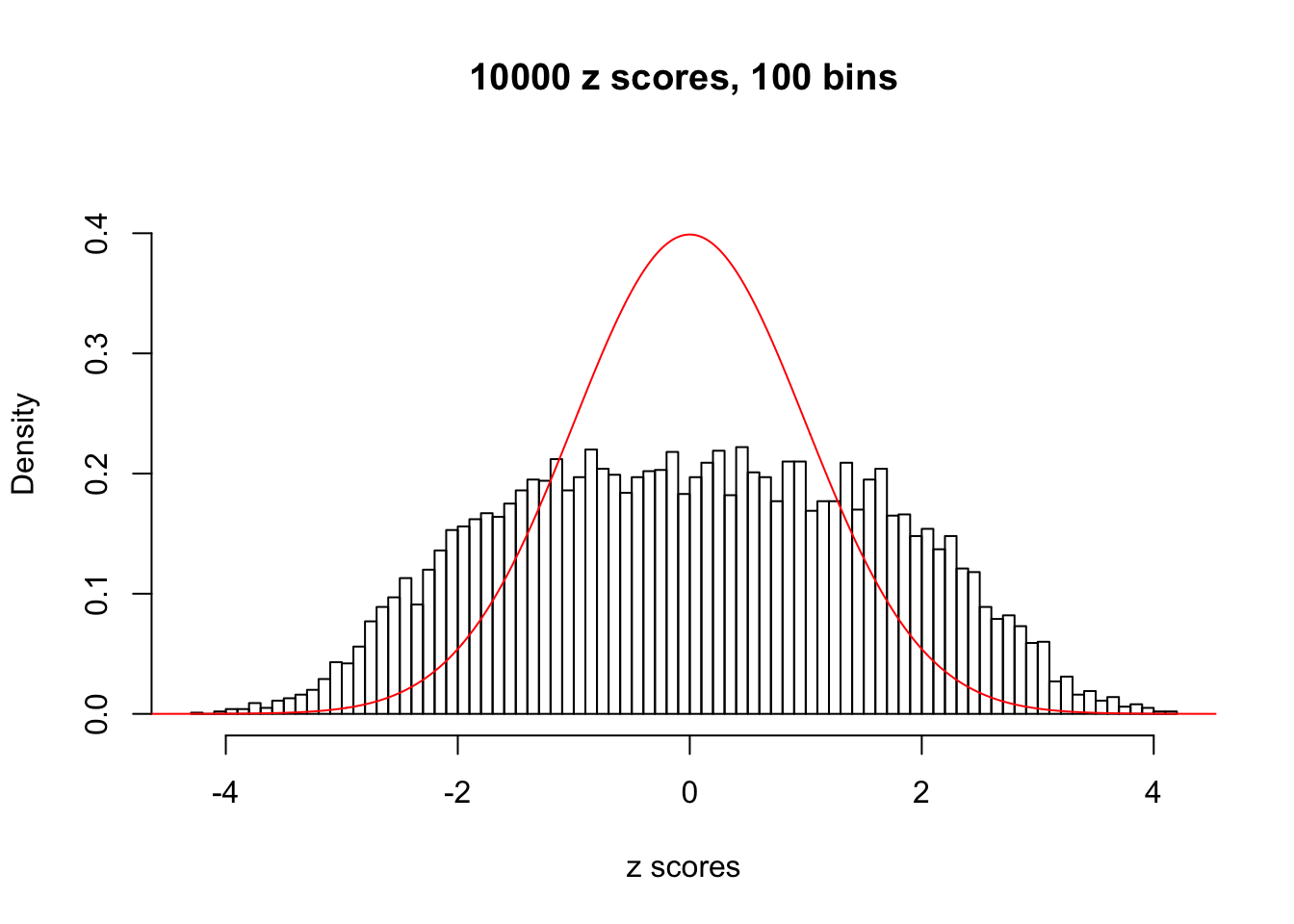


N0. 8 : Data Set 56 ; Number of False Discoveries: 35 ; pihat0 = 0.03811803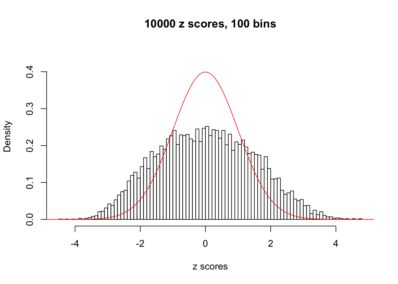


N0. 9 : Data Set 840 ; Number of False Discoveries: 28 ; pihat0 = 0.01433503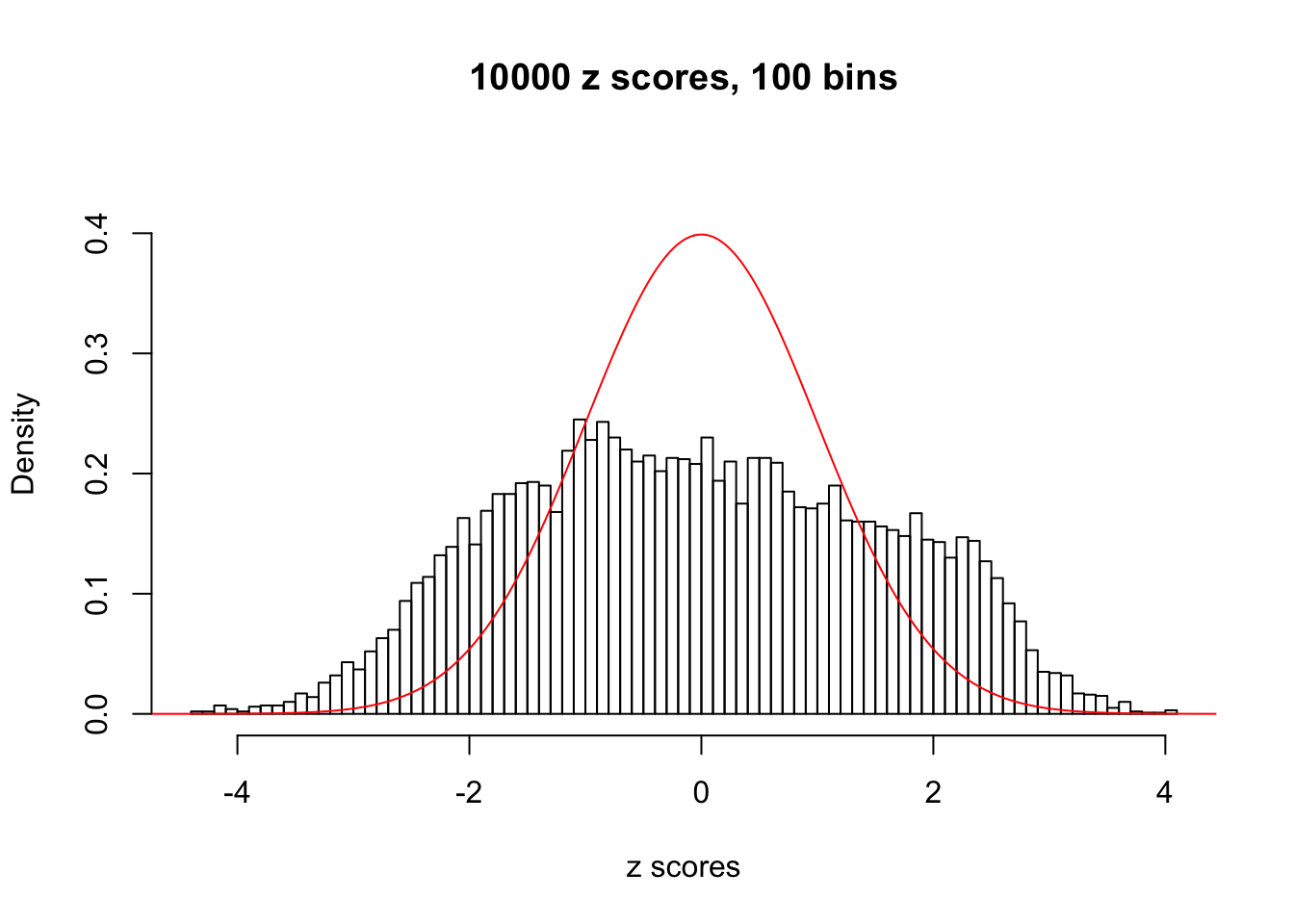


N0. 10 : Data Set 858 ; Number of False Discoveries: 16 ; pihat0 = 0.01340537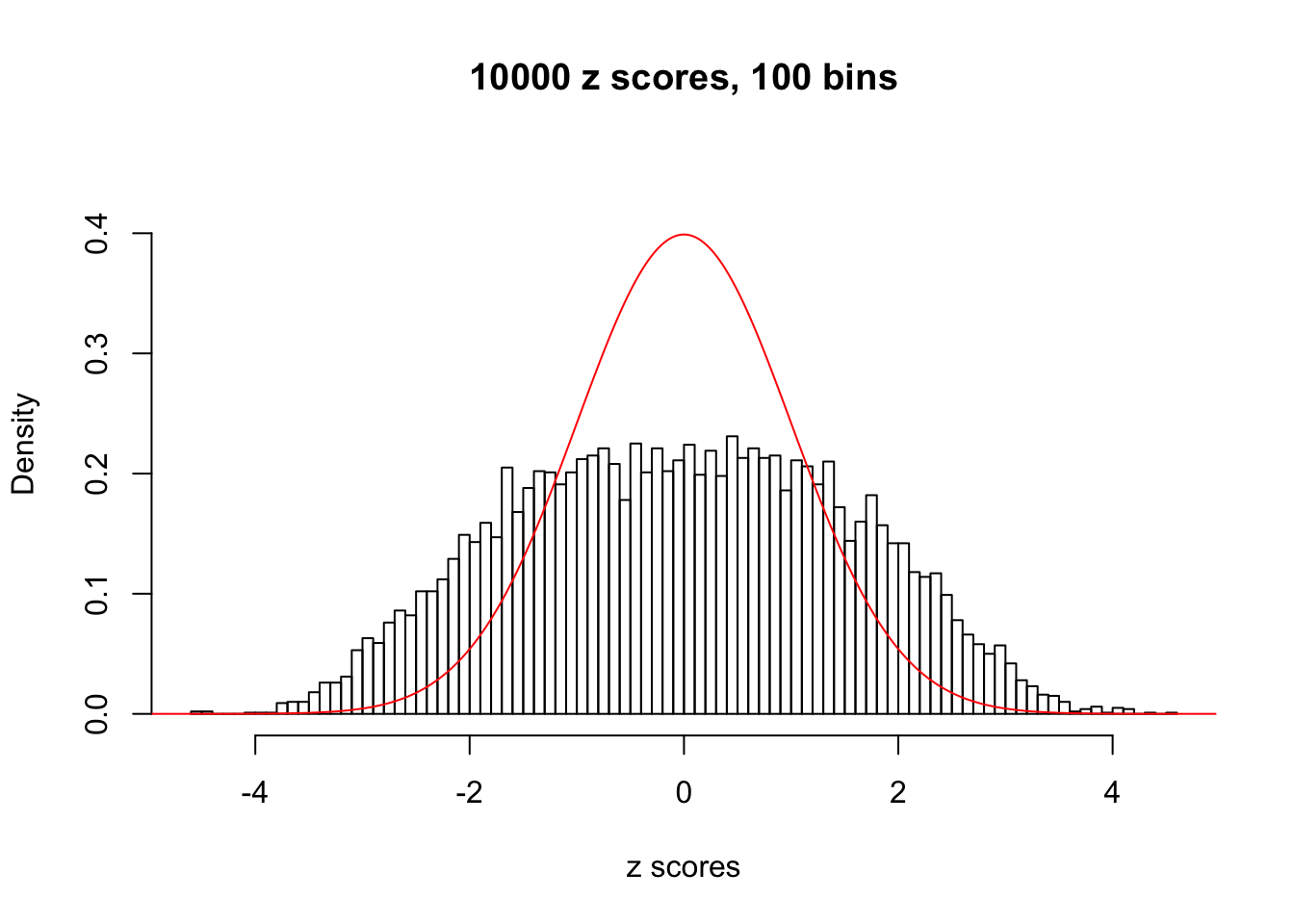


N0. 11 : Data Set 771 ; Number of False Discoveries: 12 ; pihat0 = 0.04069309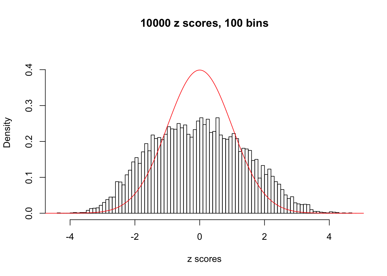


N0. 12 : Data Set 389 ; Number of False Discoveries: 11 ; pihat0 = 0.02694463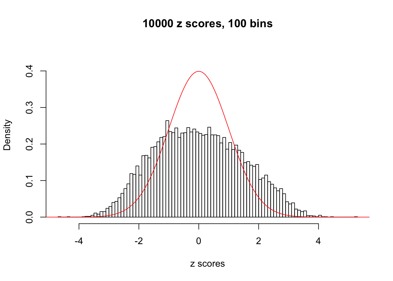


N0. 13 : Data Set 485 ; Number of False Discoveries: 9 ; pihat0 = 0.03190266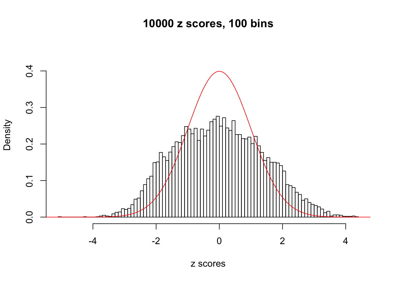


N0. 14 : Data Set 77 ; Number of False Discoveries: 7 ; pihat0 = 0.0240265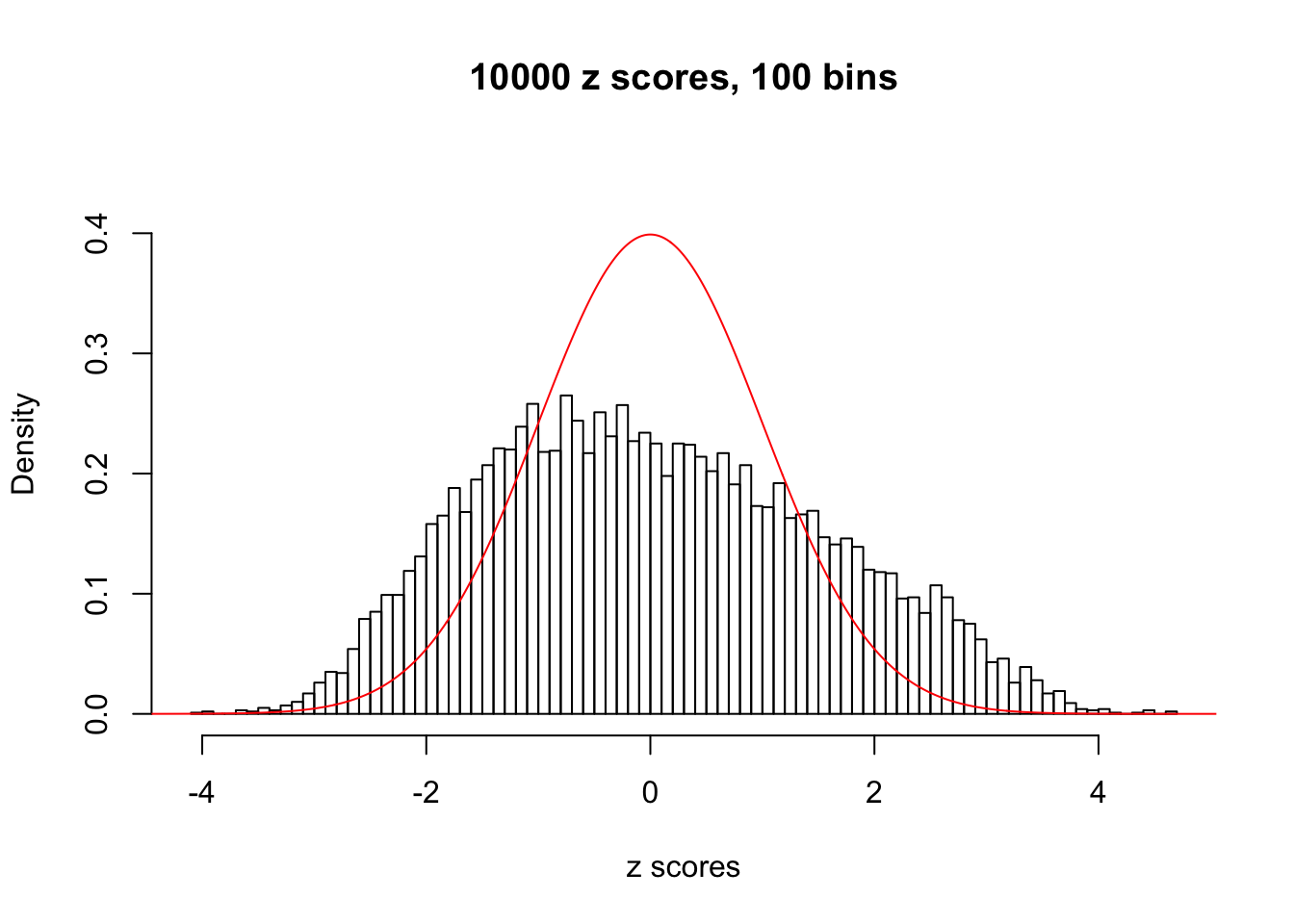


N0. 15 : Data Set 503 ; Number of False Discoveries: 7 ; pihat0 = 0.1290869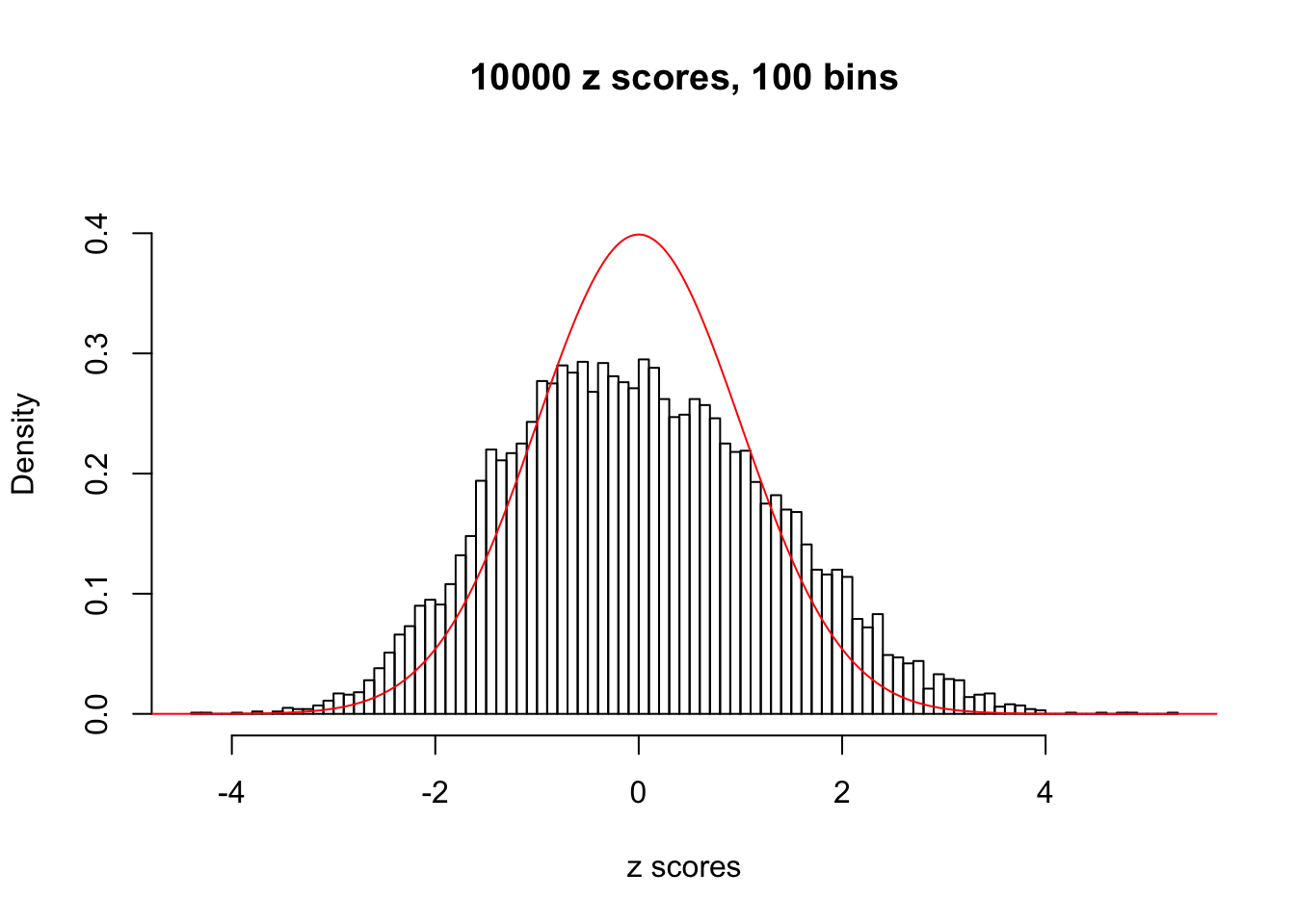


N0. 16 : Data Set 984 ; Number of False Discoveries: 7 ; pihat0 = 0.04373679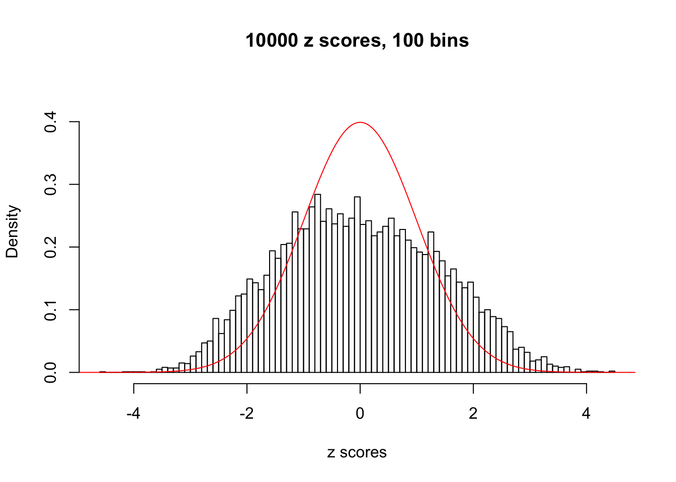


N0. 17 : Data Set 360 ; Number of False Discoveries: 6 ; pihat0 = 0.01242637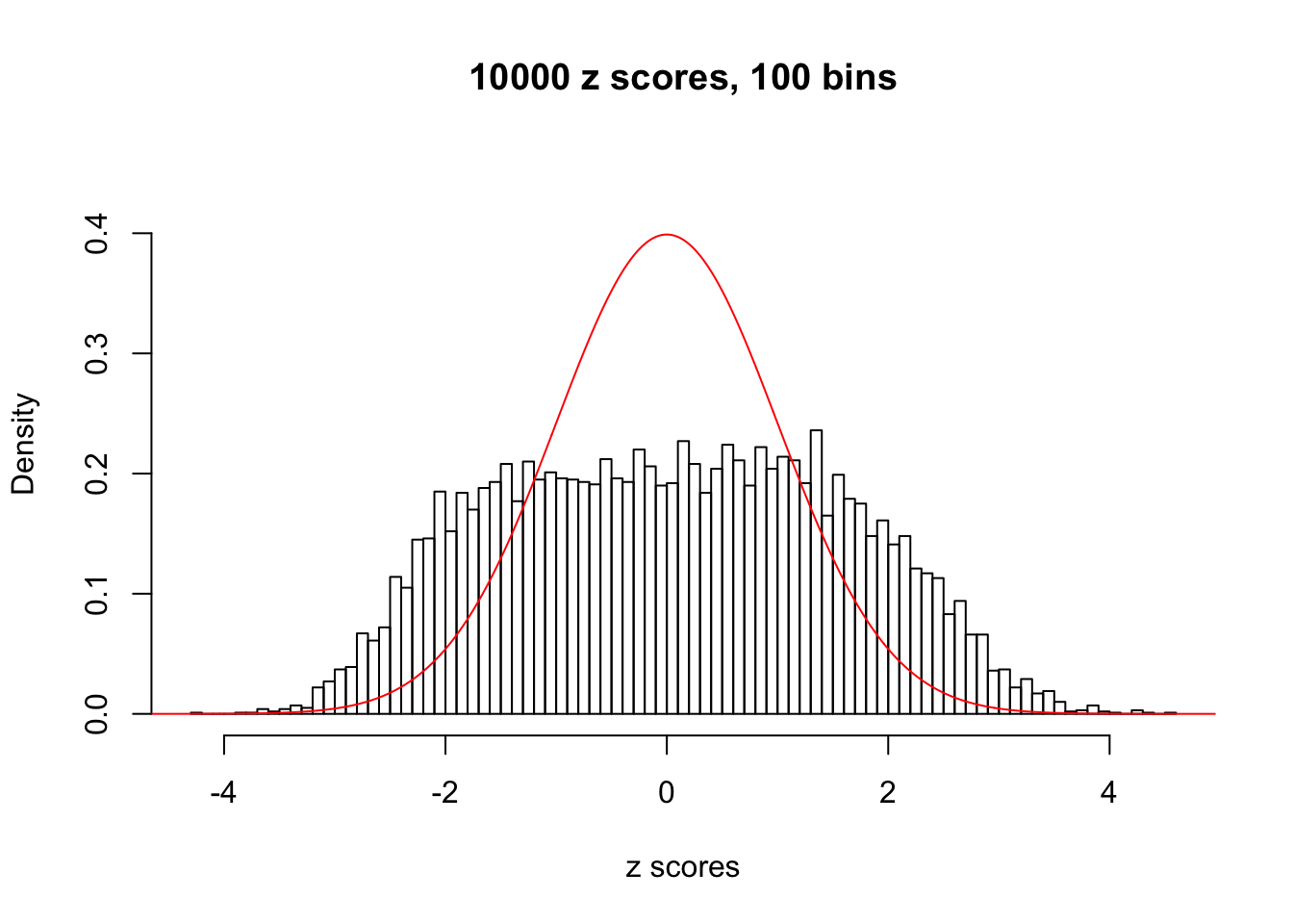


N0. 18 : Data Set 522 ; Number of False Discoveries: 4 ; pihat0 = 0.02361336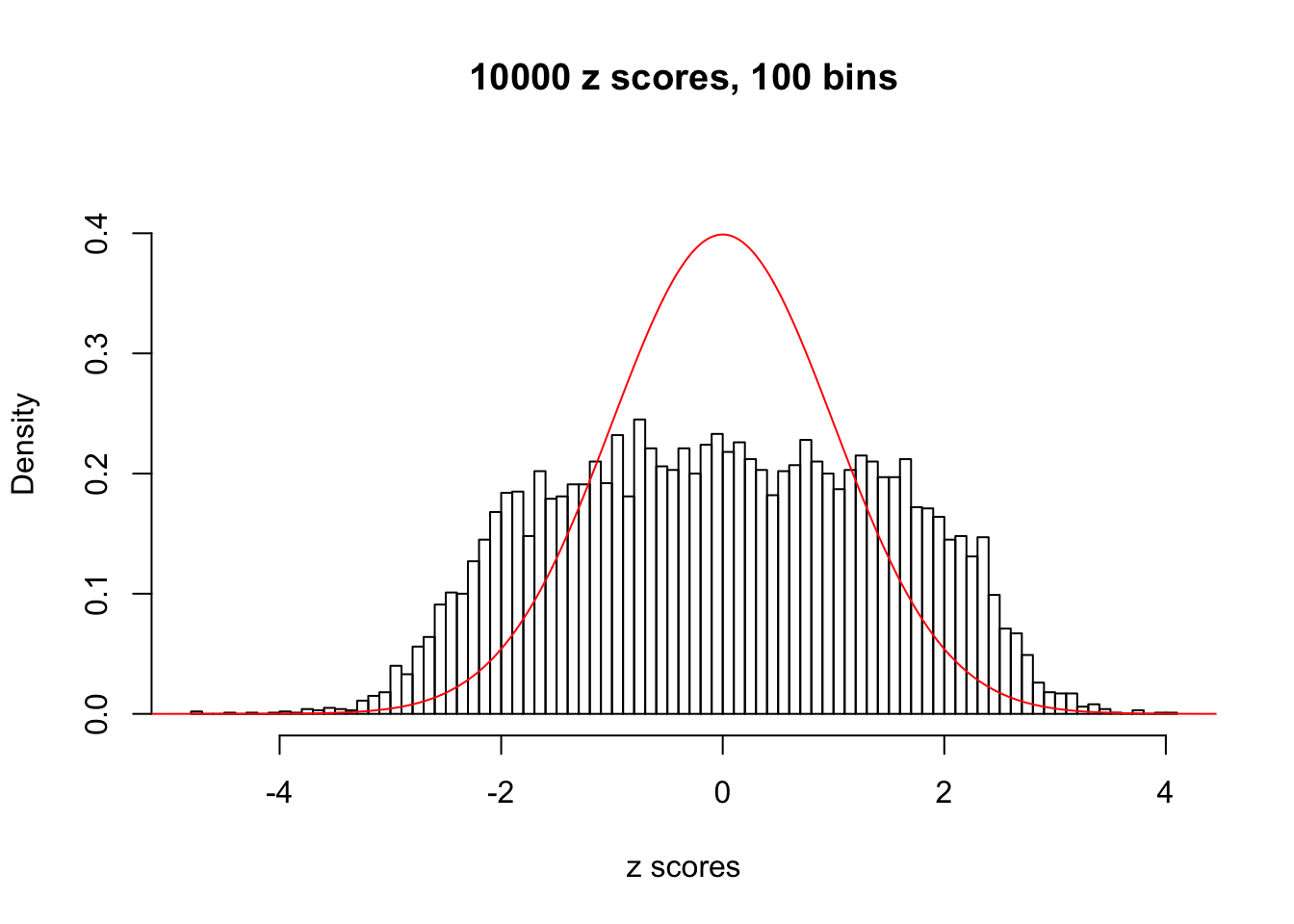


N0. 19 : Data Set 51 ; Number of False Discoveries: 3 ; pihat0 = 0.07300305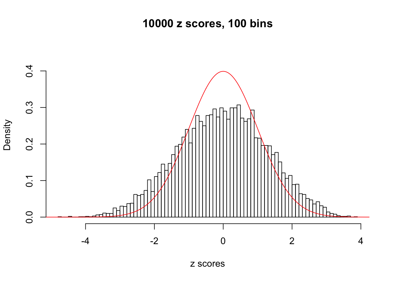


N0. 20 : Data Set 316 ; Number of False Discoveries: 3 ; pihat0 = 0.1078068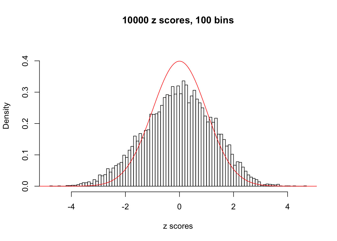


N0. 21 : Data Set 663 ; Number of False Discoveries: 3 ; pihat0 = 0.1696198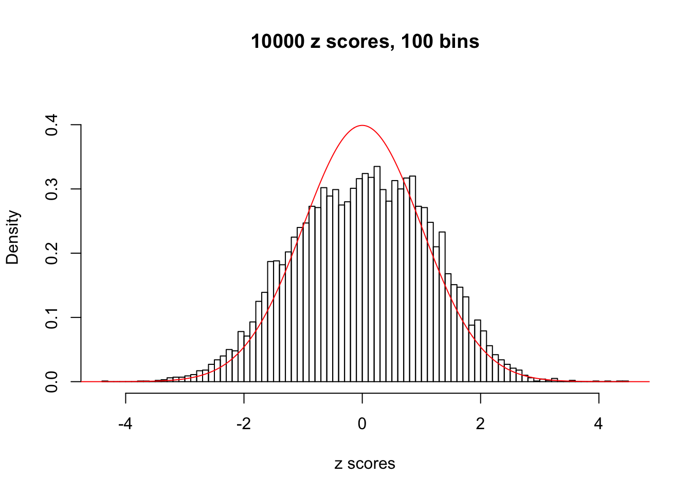


N0. 22 : Data Set 274 ; Number of False Discoveries: 2 ; pihat0 = 0.08298182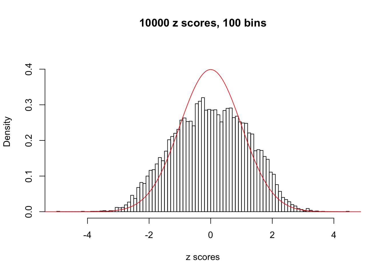


N0. 23 : Data Set 901 ; Number of False Discoveries: 2 ; pihat0 = 0.9997685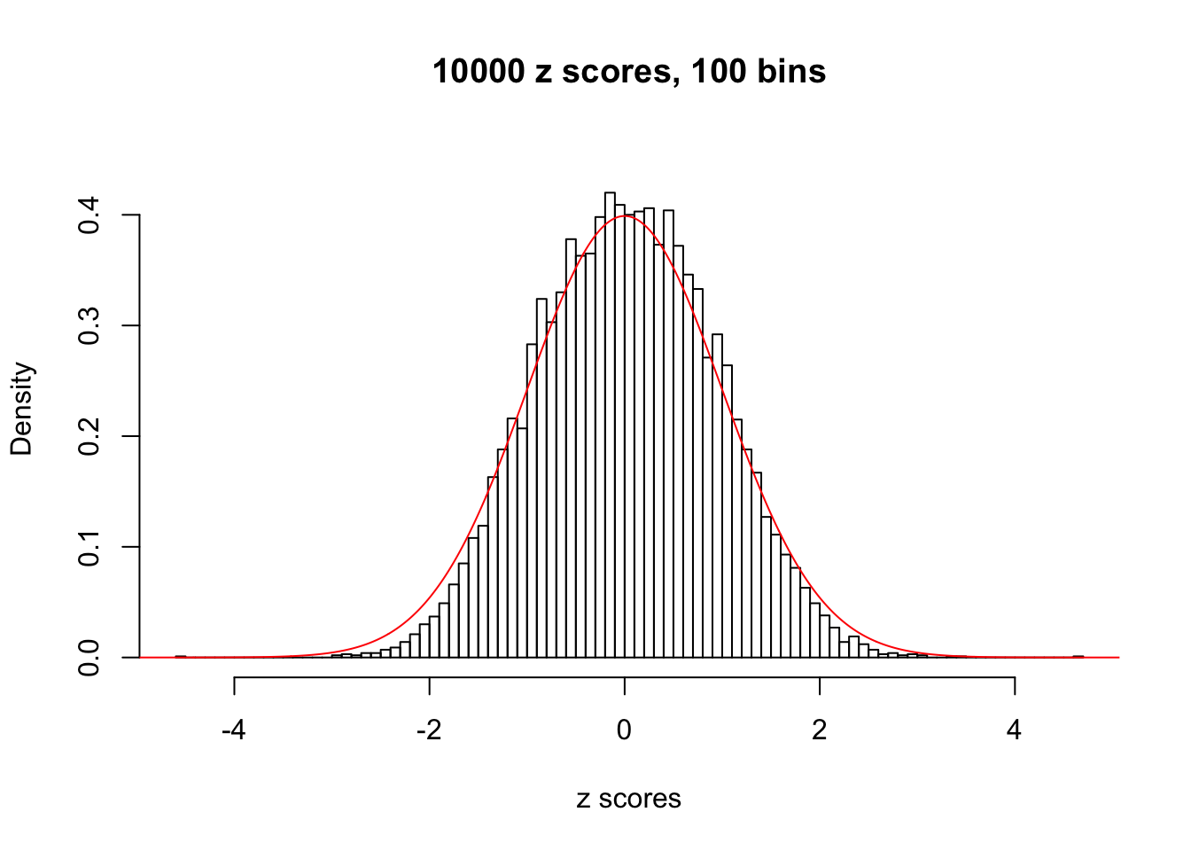


N0. 24 : Data Set 912 ; Number of False Discoveries: 2 ; pihat0 = 0.08821883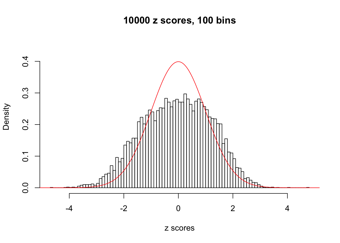


N0. 25 : Data Set 22 ; Number of False Discoveries: 1 ; pihat0 = 0.0328122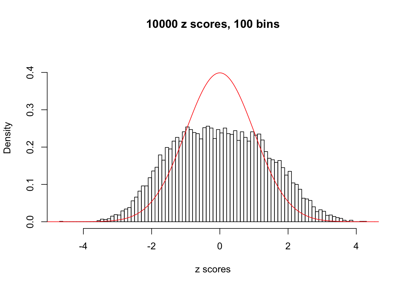


N0. 26 : Data Set 31 ; Number of False Discoveries: 1 ; pihat0 = 0.09577454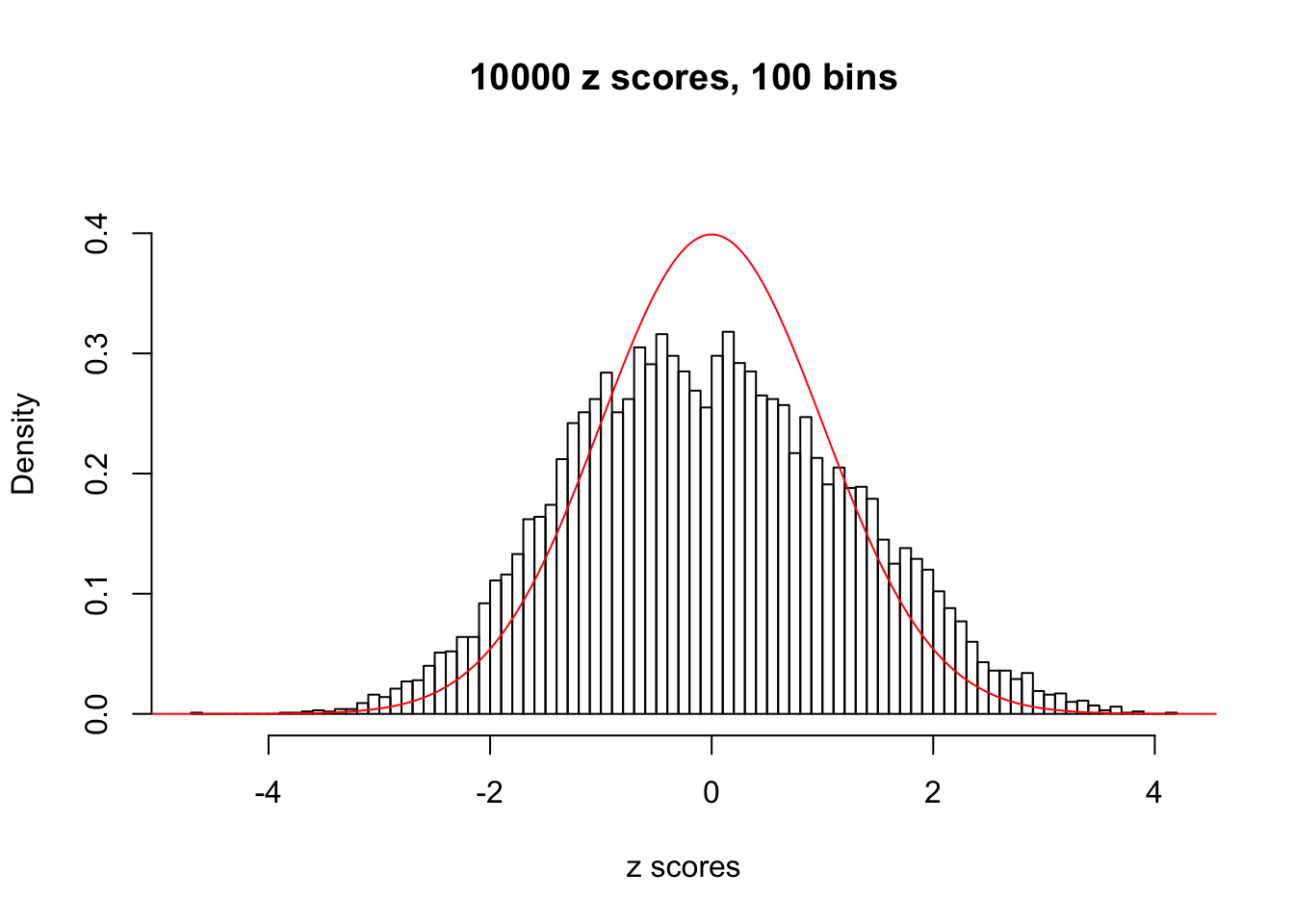


N0. 27 : Data Set 187 ; Number of False Discoveries: 1 ; pihat0 = 0.6662317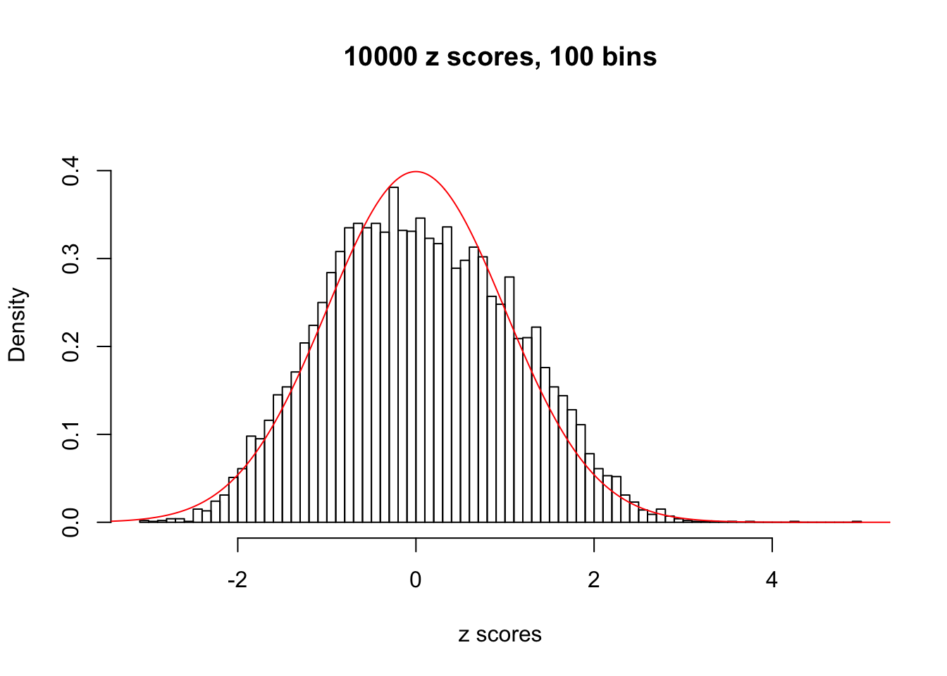


N0. 28 : Data Set 248 ; Number of False Discoveries: 1 ; pihat0 = 0.4583919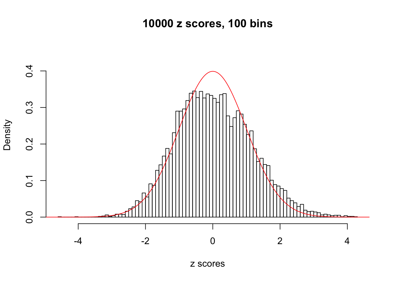


N0. 29 : Data Set 269 ; Number of False Discoveries: 1 ; pihat0 = 0.03060497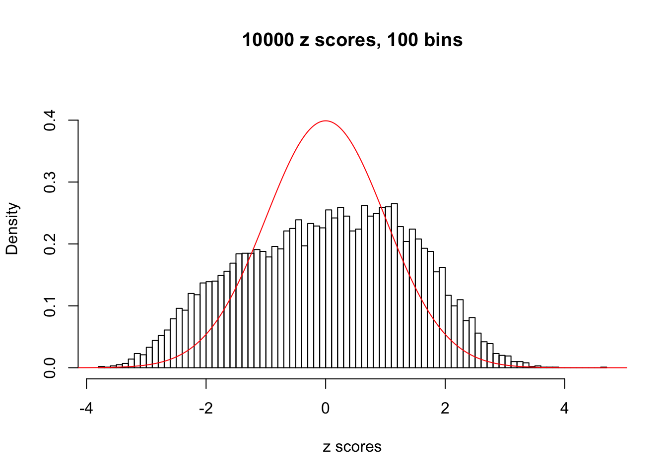


N0. 30 : Data Set 285 ; Number of False Discoveries: 1 ; pihat0 = 0.5178013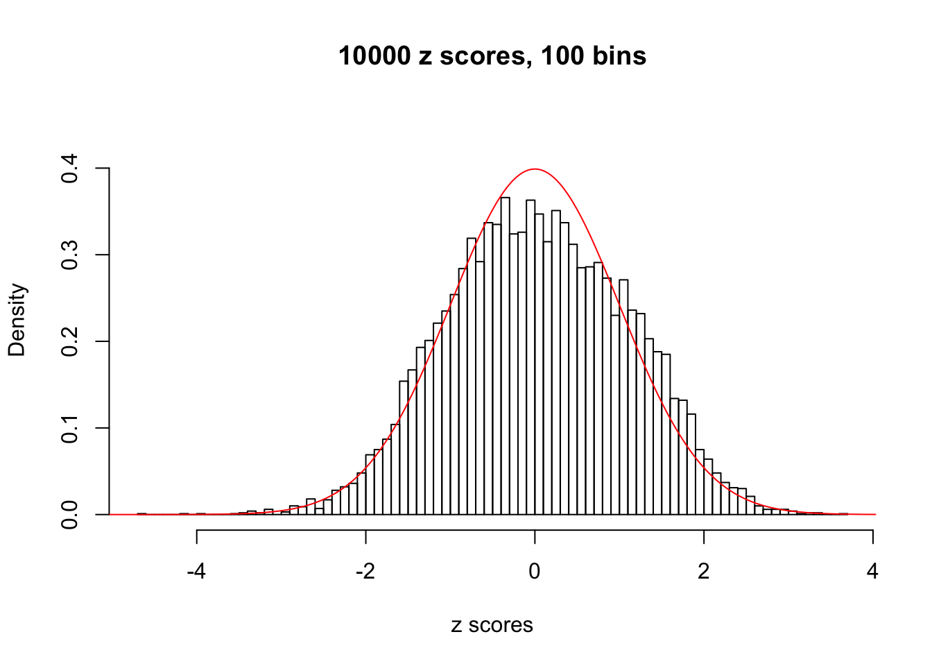


N0. 31 : Data Set 403 ; Number of False Discoveries: 1 ; pihat0 = 0.03166538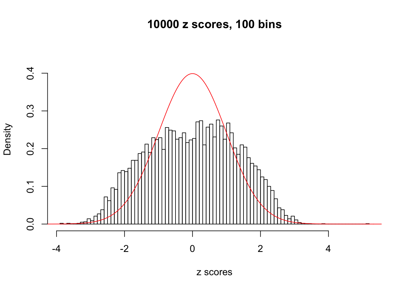


N0. 32 : Data Set 483 ; Number of False Discoveries: 1 ; pihat0 = 0.9998828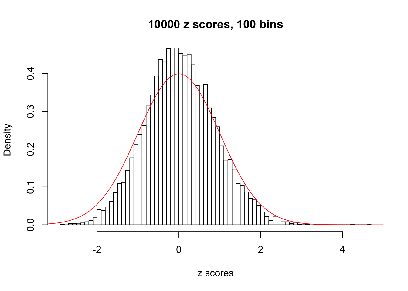


N0. 33 : Data Set 501 ; Number of False Discoveries: 1 ; pihat0 = 0.09362328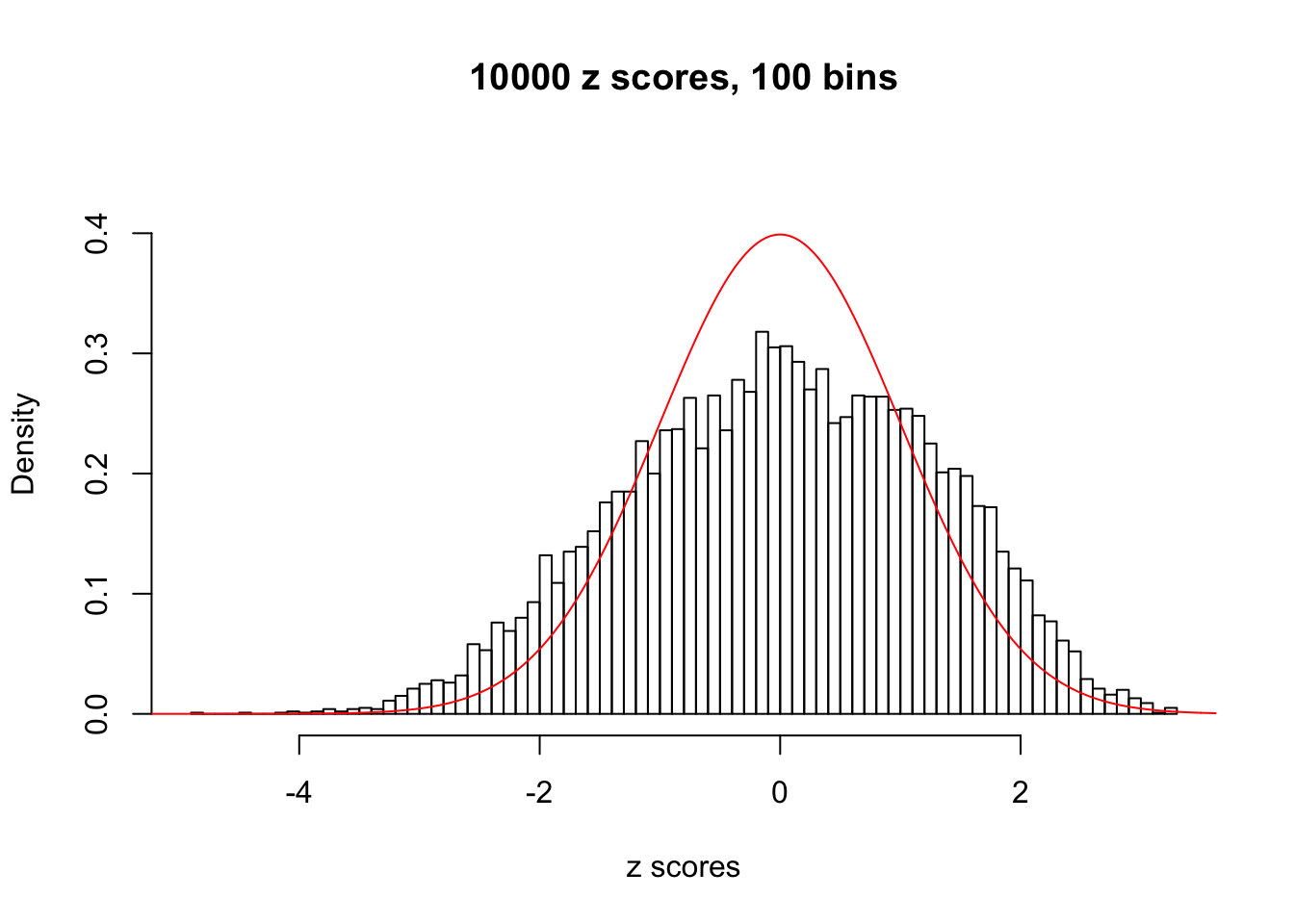


N0. 34 : Data Set 530 ; Number of False Discoveries: 1 ; pihat0 = 0.4320548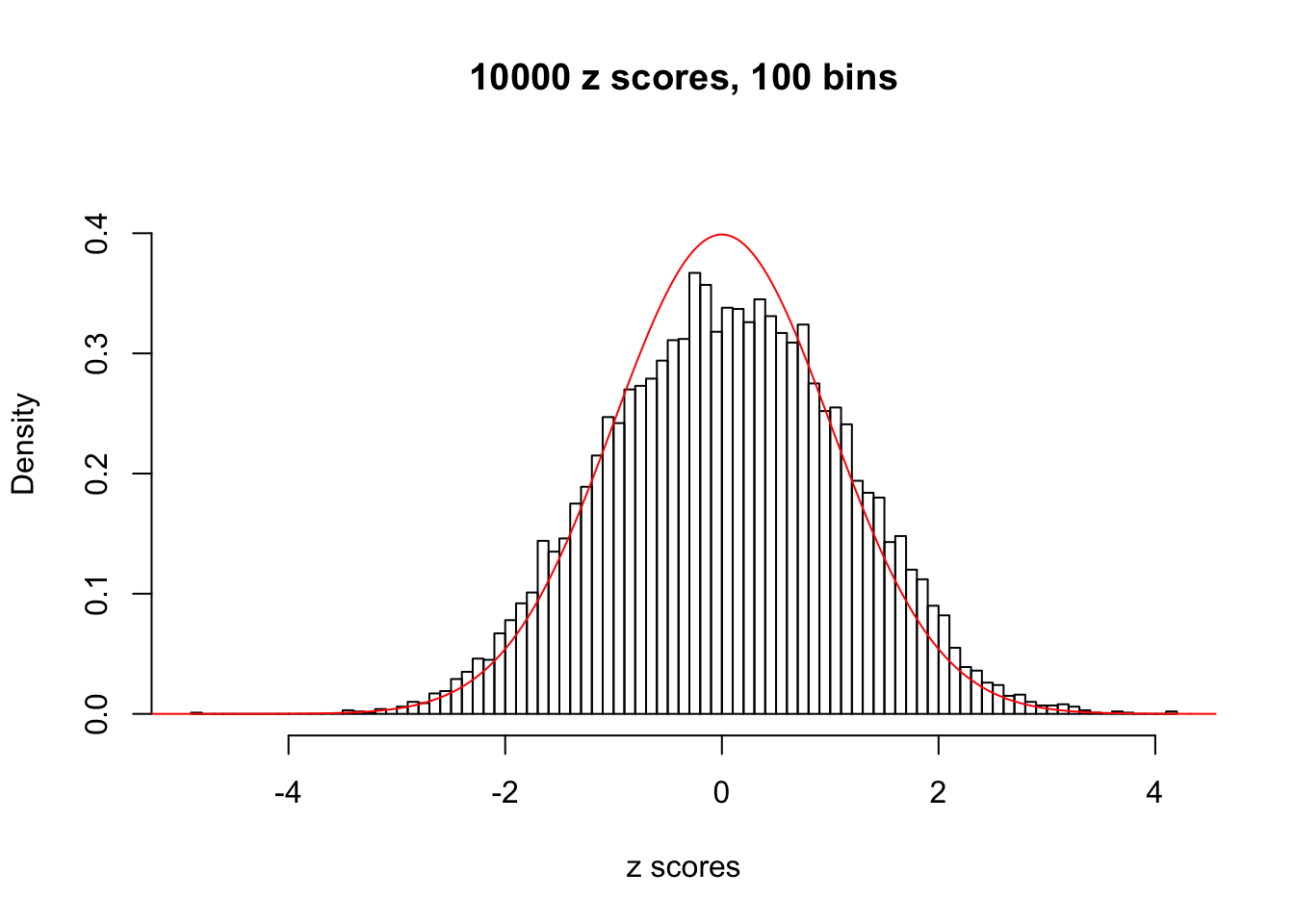


N0. 35 : Data Set 574 ; Number of False Discoveries: 1 ; pihat0 = 0.3723755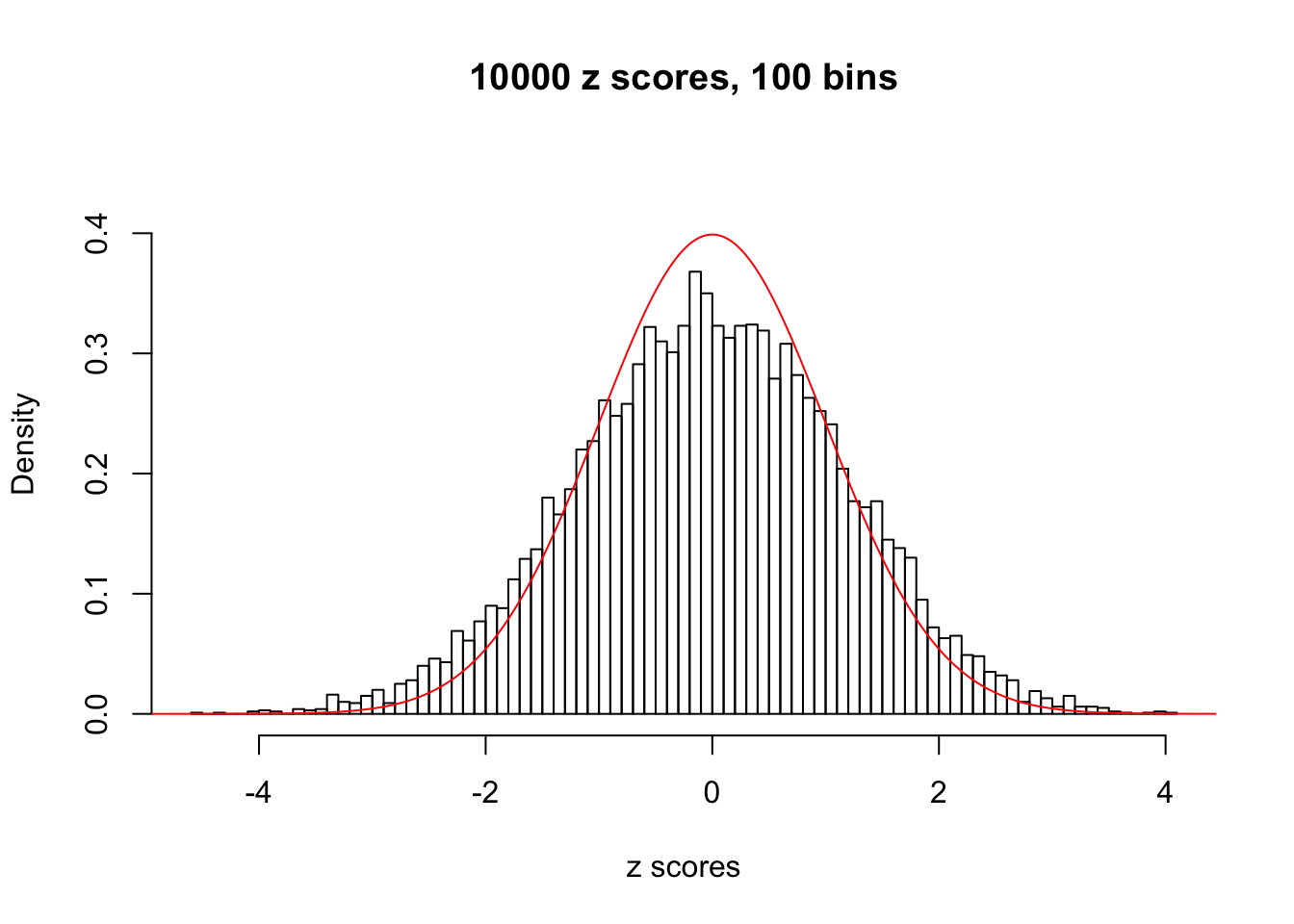


N0. 36 : Data Set 575 ; Number of False Discoveries: 1 ; pihat0 = 0.03307994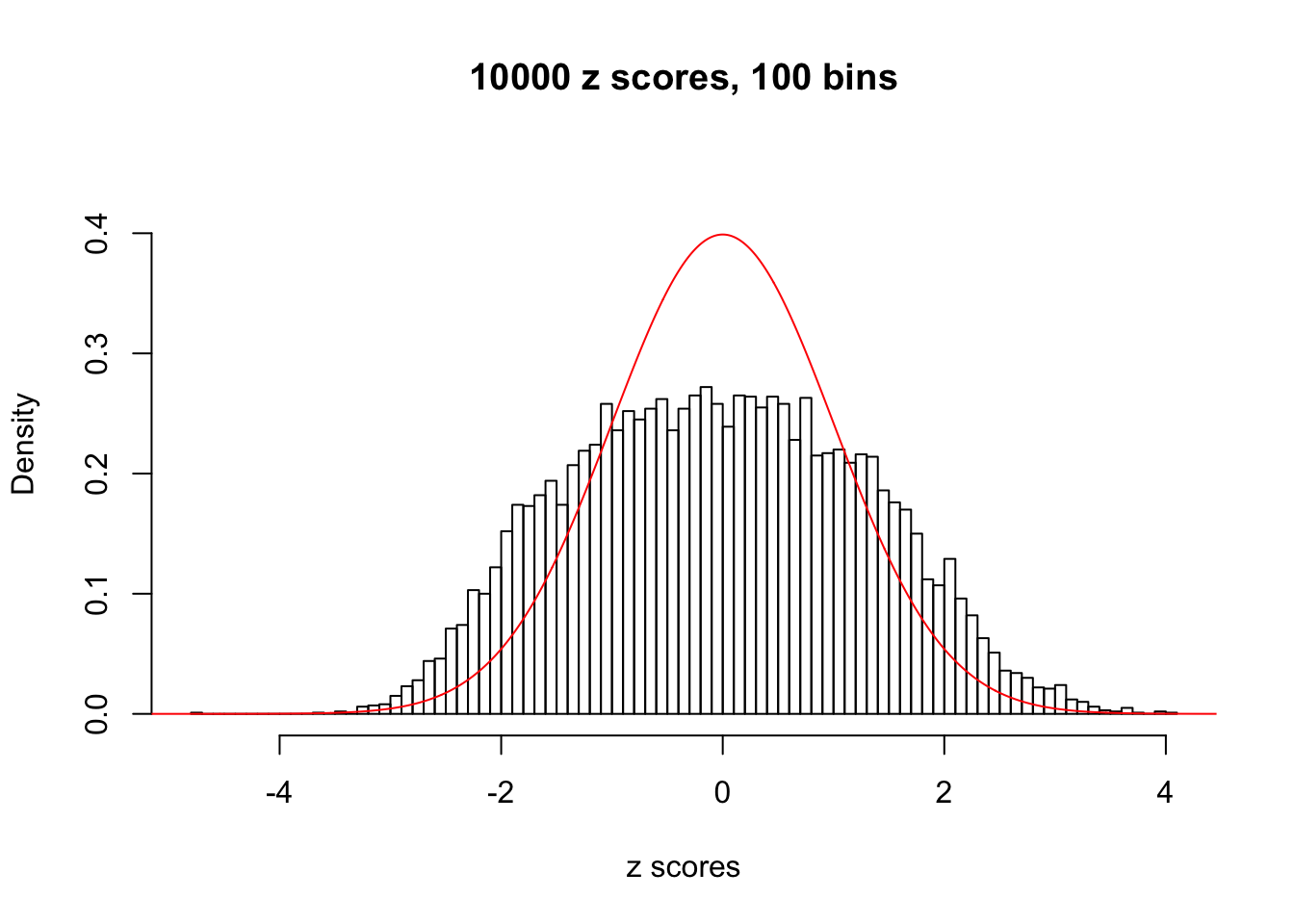


N0. 37 : Data Set 643 ; Number of False Discoveries: 1 ; pihat0 = 0.160838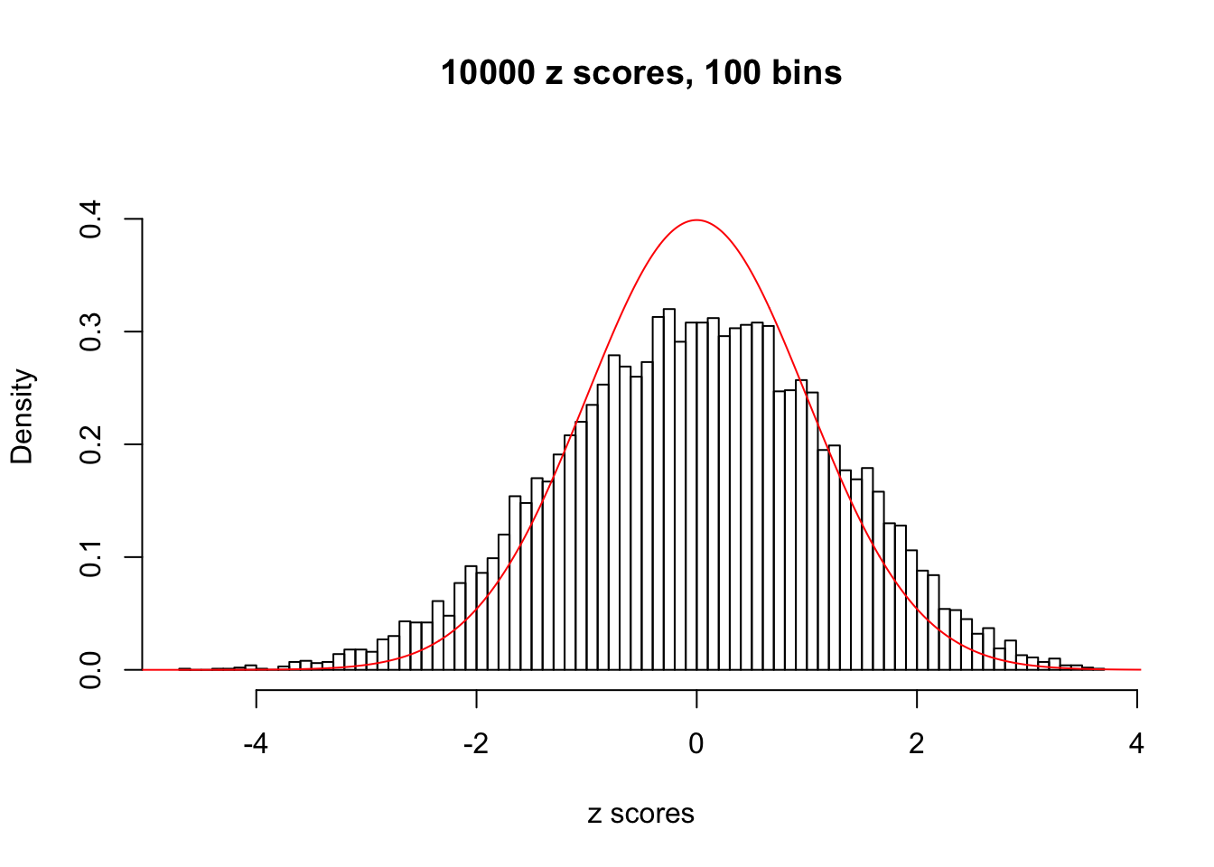


N0. 38 : Data Set 769 ; Number of False Discoveries: 1 ; pihat0 = 0.1227421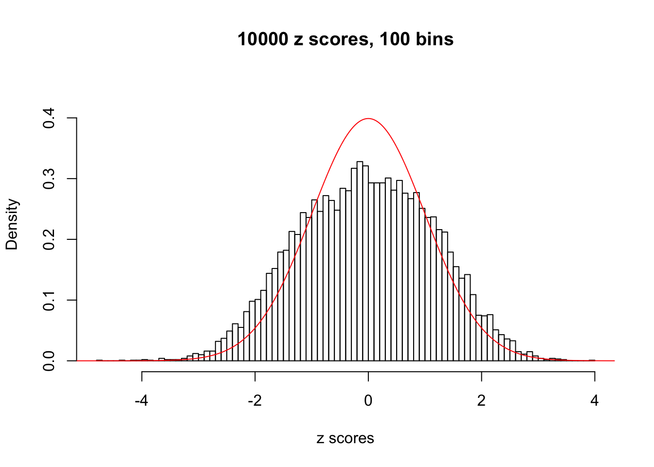


N0. 39 : Data Set 778 ; Number of False Discoveries: 1 ; pihat0 = 0.05117821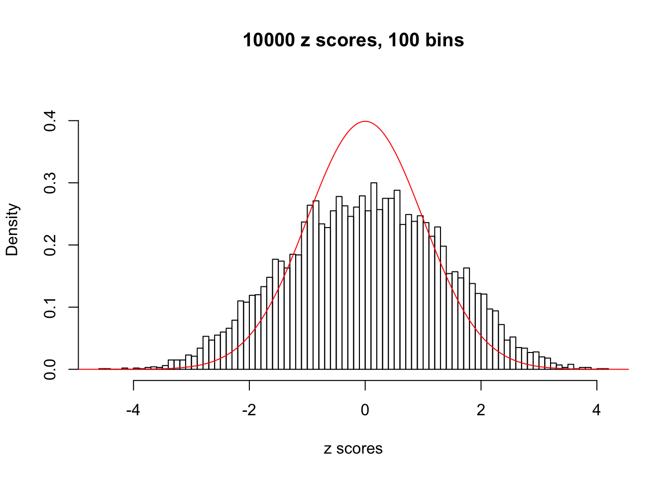


N0. 40 : Data Set 817 ; Number of False Discoveries: 1 ; pihat0 = 1

N0. 41 : Data Set 837 ; Number of False Discoveries: 1 ; pihat0 = 0.828704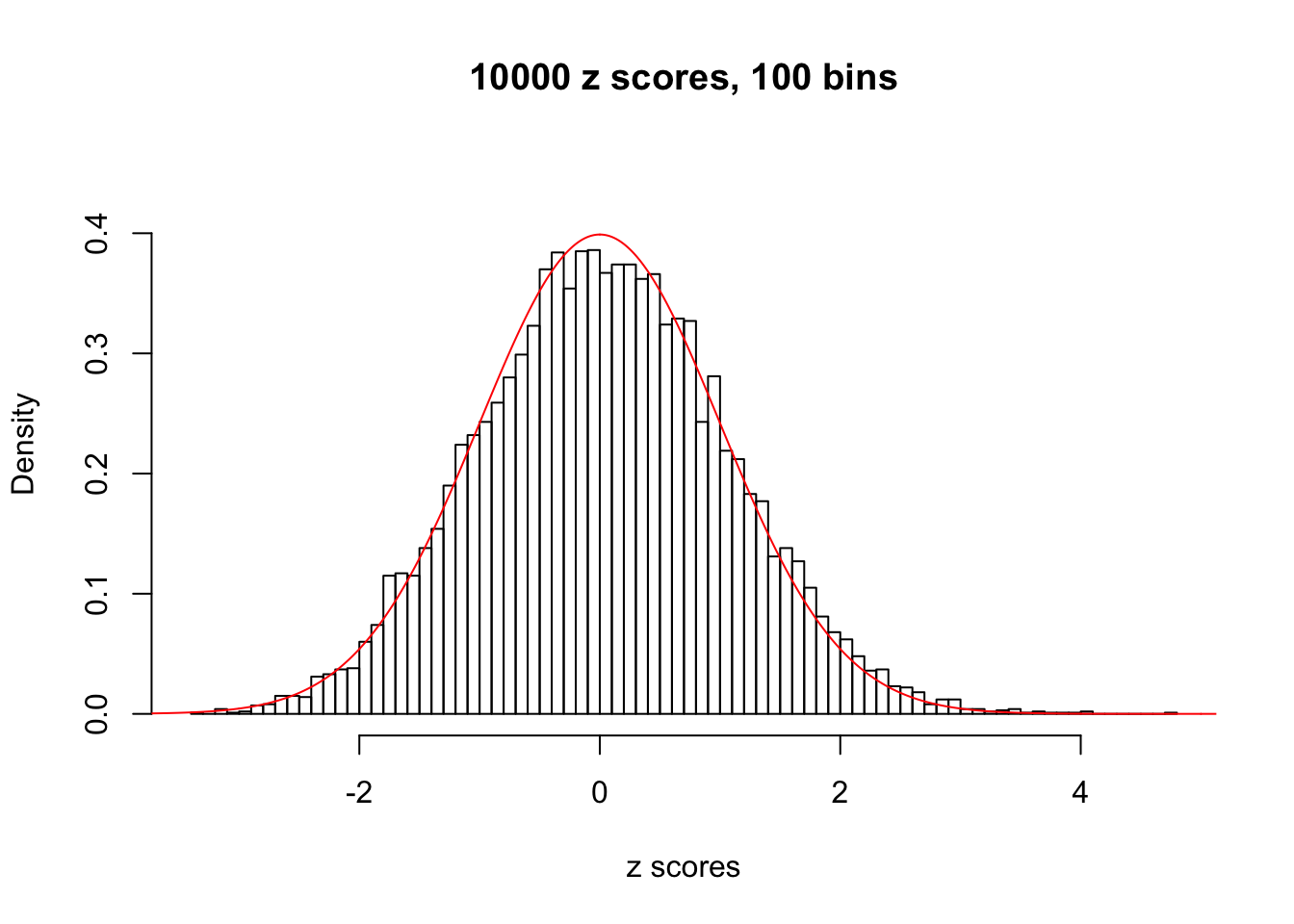


N0. 42 : Data Set 897 ; Number of False Discoveries: 1 ; pihat0 = 0.7555982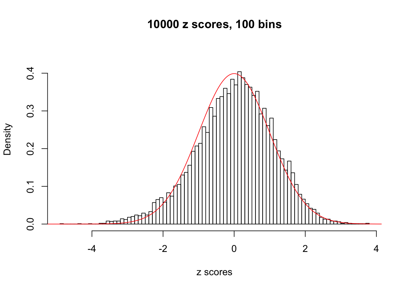


N0. 43 : Data Set 923 ; Number of False Discoveries: 1 ; pihat0 = 0.01590919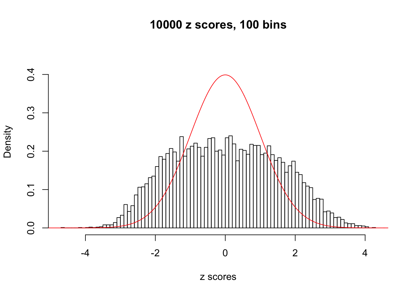


N0. 44 : Data Set 955 ; Number of False Discoveries: 1 ; pihat0 = 0.9998902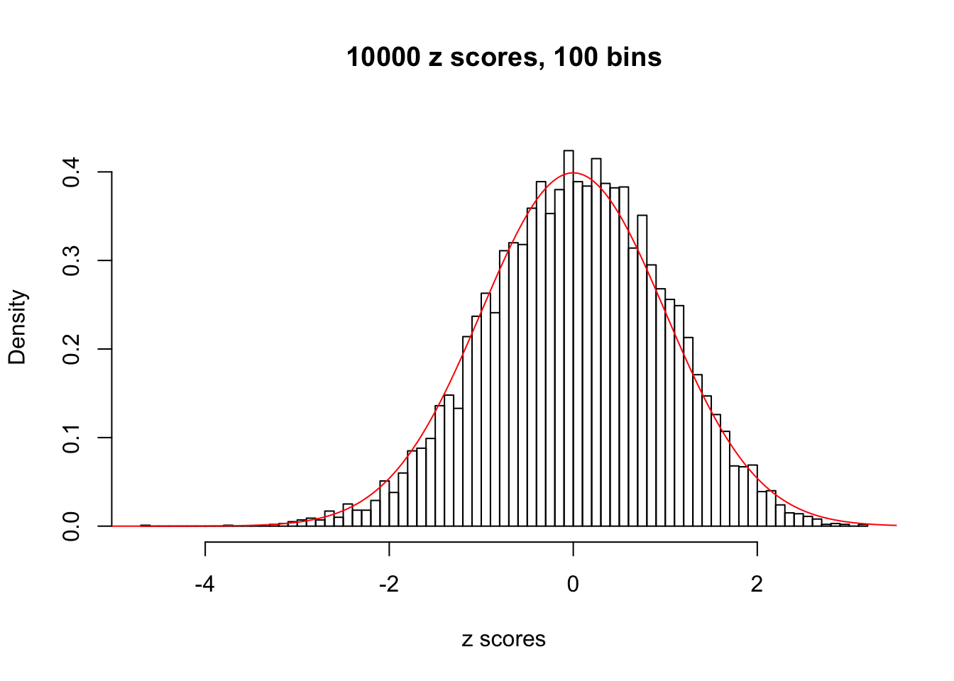


N0. 45 : Data Set 971 ; Number of False Discoveries: 1 ; pihat0 = 0.1368012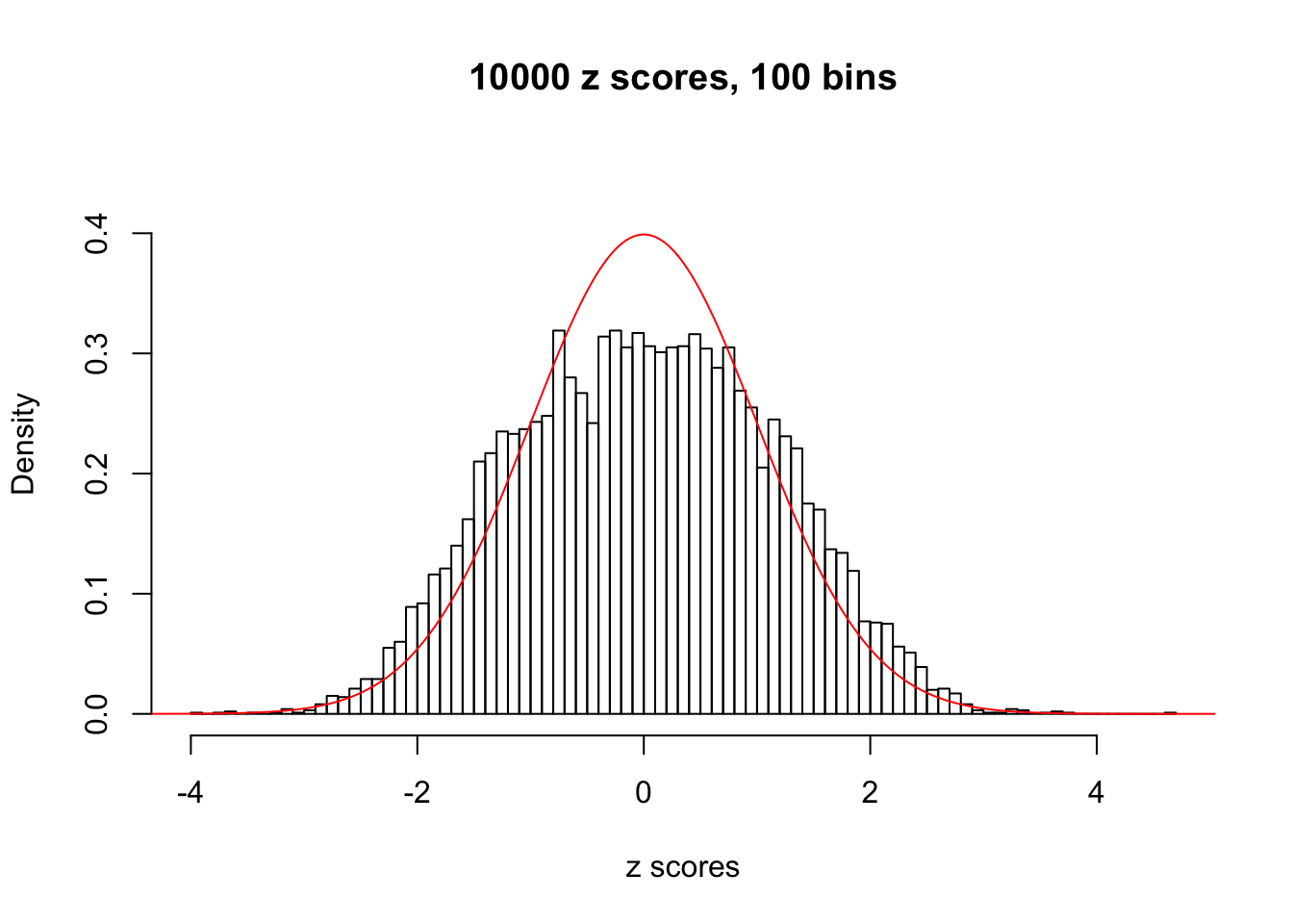


N0. 46 : Data Set 997 ; Number of False Discoveries: 1 ; pihat0 = 0.1018171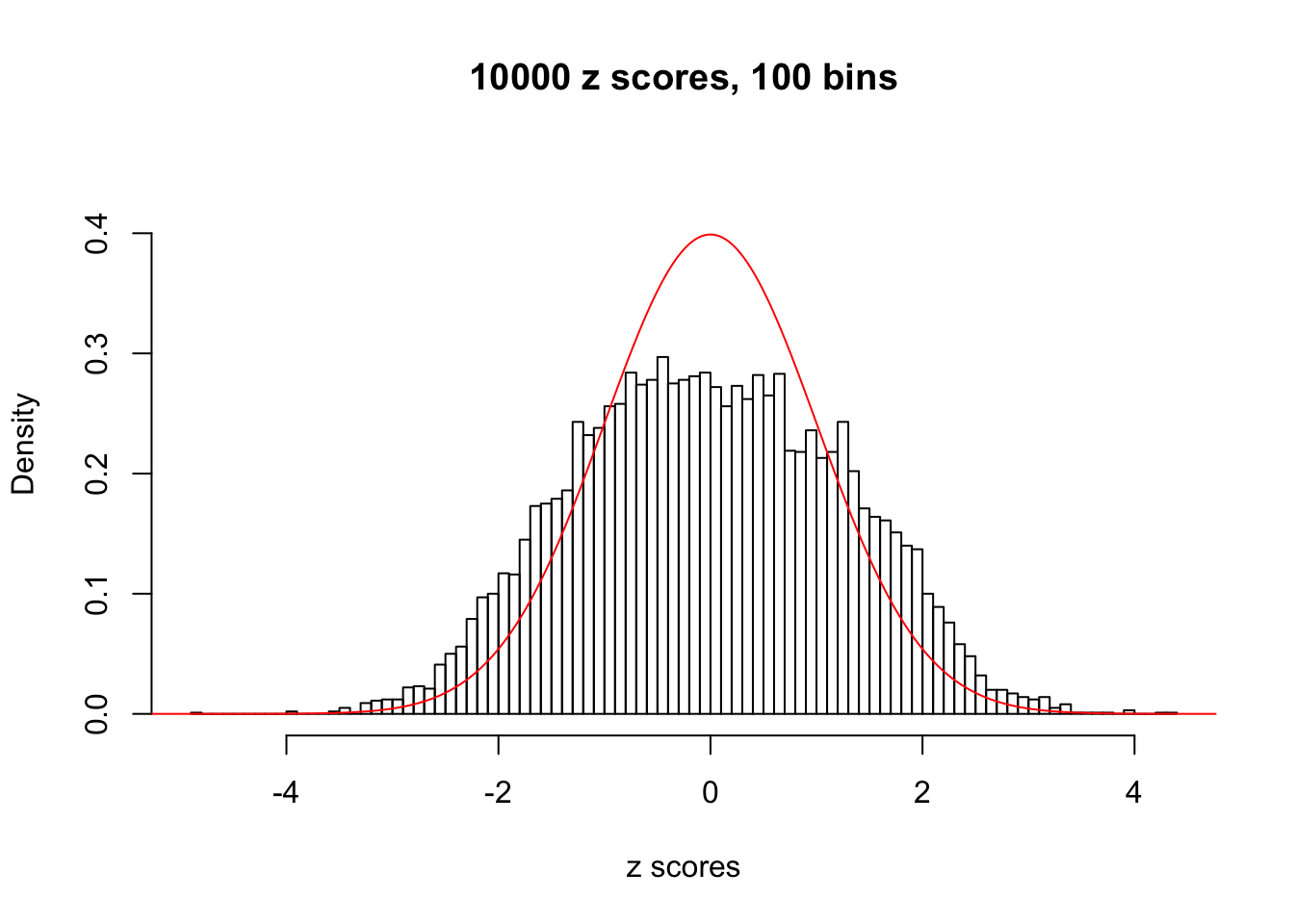


Remarks on goodness of fit
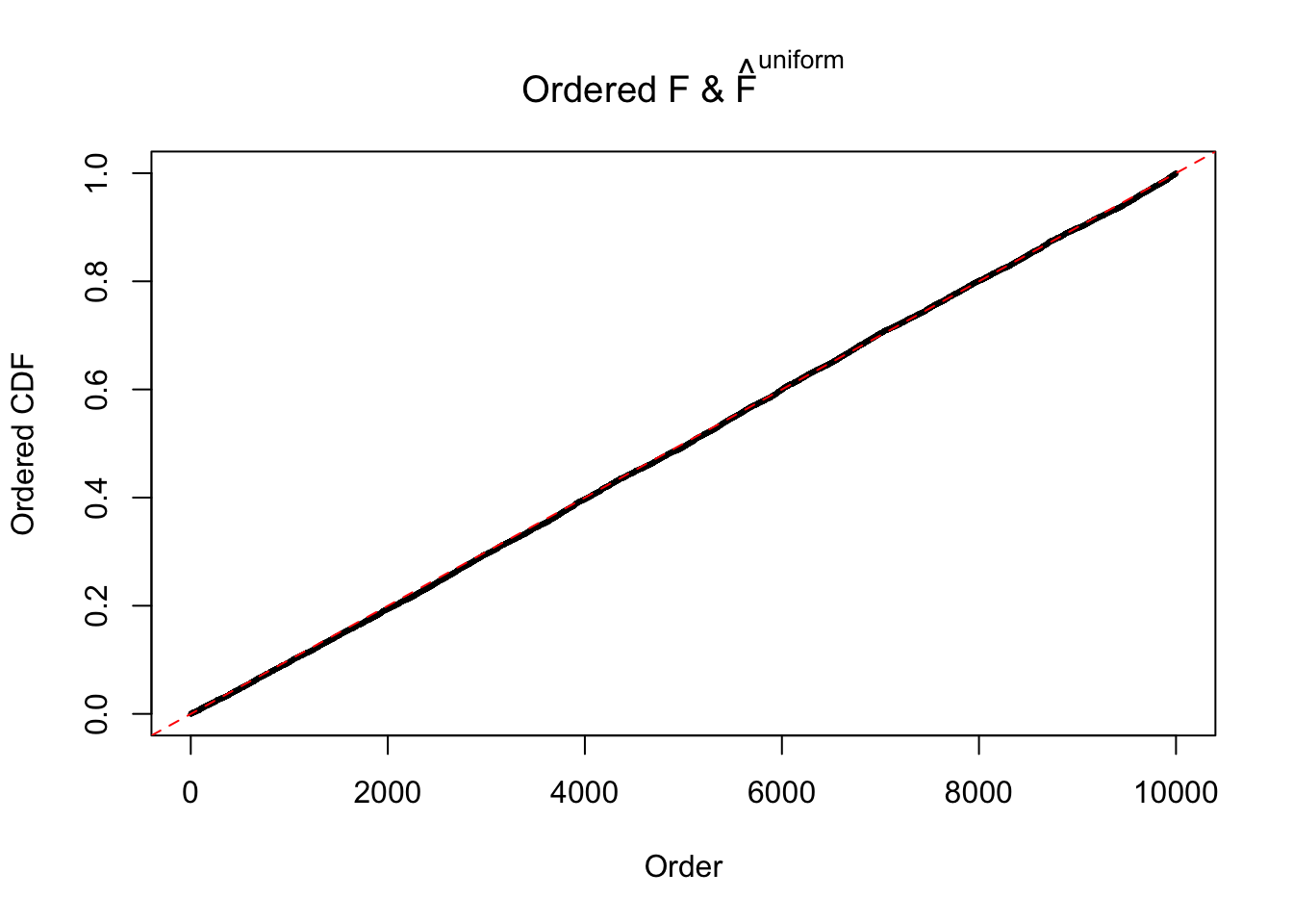
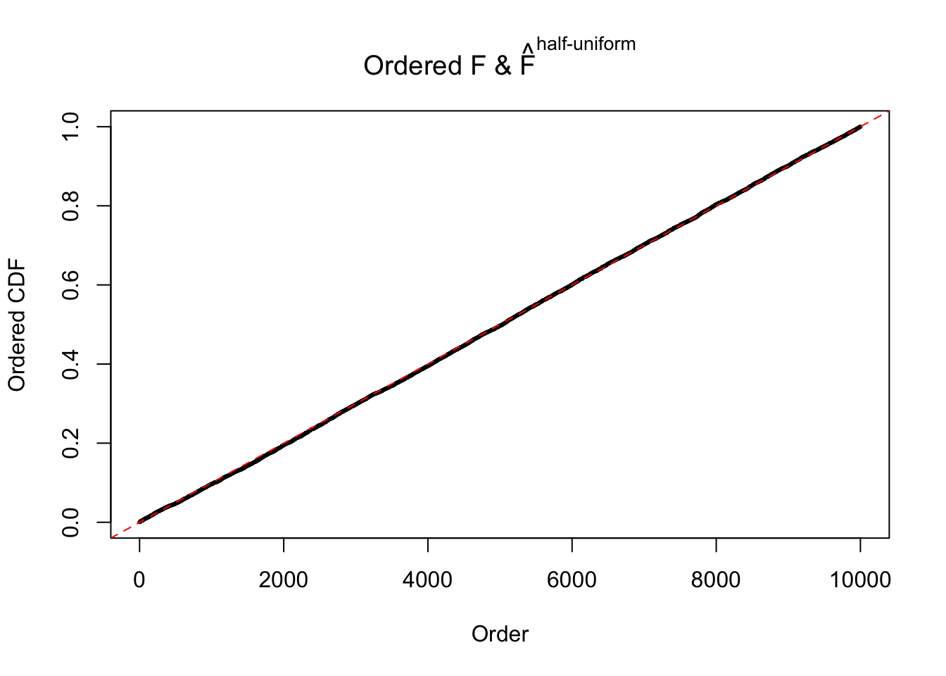
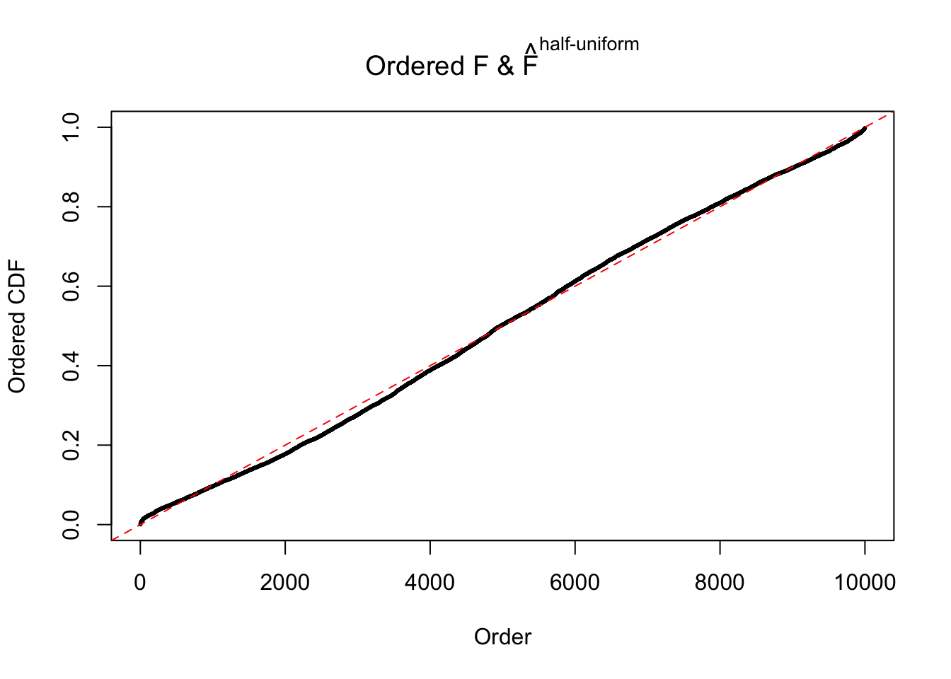
The simulation shows that oftentimes, ASH, no matter what kind of mixture prior is used, would only be able to produce a bad fit for the pseudo-effects due to correlation-induced inflation. However, occasionally, if uniform or halfuniform is used as the mixture component for the prior, the model may have a good fit, as indicated by the uniformness of \(\left\{\hat F_j\right\}\).
Session information
sessionInfo()R version 3.4.3 (2017-11-30)
Platform: x86_64-apple-darwin15.6.0 (64-bit)
Running under: macOS High Sierra 10.13.2
Matrix products: default
BLAS: /Library/Frameworks/R.framework/Versions/3.4/Resources/lib/libRblas.0.dylib
LAPACK: /Library/Frameworks/R.framework/Versions/3.4/Resources/lib/libRlapack.dylib
locale:
[1] en_US.UTF-8/en_US.UTF-8/en_US.UTF-8/C/en_US.UTF-8/en_US.UTF-8
attached base packages:
[1] stats graphics grDevices utils datasets methods base
loaded via a namespace (and not attached):
[1] compiler_3.4.3 backports_1.1.2 magrittr_1.5 rprojroot_1.3-1
[5] tools_3.4.3 htmltools_0.3.6 yaml_2.1.16 Rcpp_0.12.14
[9] stringi_1.1.6 rmarkdown_1.8 knitr_1.17 git2r_0.20.0
[13] stringr_1.2.0 digest_0.6.13 evaluate_0.10.1This R Markdown site was created with workflowr