Posterior Inference with Gaussian Derivative Likelihood: Model and Result
Lei Sun
2017-06-14
Last updated: 2017-12-21
Code version: 6e42447
GD-ASH Model
Recall the typical GD-ASH model is
\[ \begin{array}{l} \beta_j \sim \sum\pi_k N\left(0, \sigma_k^2\right) \ ;\\ \hat\beta_j = \beta_j + \hat s_j z_j \ ;\\ z_j \sim N\left(0, 1\right), \text{ correlated} \ . \end{array} \] Then we are fitting the empirical distribution of \(z\) with Gaussian derivatives
\[ f(z) = \sum w_l\frac{1}{\sqrt{l!}}\varphi^{(l)}(z) \ . \] Therefore, in essence, we are changing the likelihood of \(\hat\beta_j | \hat s_j, \beta_j\) from correlated \(N\left(\beta_j, \hat s_j^2\right)\) to independent \(\frac{1}{\hat s_j}f\left(\frac{\hat\beta_j - \beta_j}{\hat s_j}\right)\), which using Gaussian derivatives is
\[ \frac{1}{\hat s_j}\sum w_l \frac{1}{\sqrt{l!}} \varphi^{(l)}\left(\frac{\hat\beta_j - \beta_j}{\hat s_j}\right) \ . \] Note that when \(f = \varphi\) it becomes the independent \(N\left(\beta_j, \hat s_j^2\right)\) case.
GD-Lik Model
Therefore, if we use Gaussian derivatives instead of Gaussian as the likelihood, the posterior distribution of \(\beta_j | \hat s_j, \hat\beta_j\) should be
\[ \begin{array}{rcl} f\left(\beta_j \mid \hat s_j, \hat\beta_j\right) &=& \frac{ \displaystyle g\left(\beta_j\right) f\left(\hat\beta_j \mid \hat s_j, \beta_j \right) }{ \displaystyle\int g\left(\beta_j\right) f\left(\hat\beta_j \mid \hat s_j, \beta_j \right) d\beta_j }\\ &=& \frac{ \displaystyle \sum\pi_k\sum w_l \frac{1}{\sigma_k} \varphi\left(\frac{\beta_j - \mu_k}{\sigma_k}\right) \frac{1}{\hat s_j} \frac{1}{\sqrt{l!}} \varphi^{(l)}\left(\frac{\hat\beta_j - \beta_j}{\hat s_j}\right) }{ \displaystyle \sum\pi_k\sum w_l \int \frac{1}{\sigma_k} \varphi\left(\frac{\beta_j - \mu_k}{\sigma_k}\right) \frac{1}{\hat s_j} \frac{1}{\sqrt{l!}} \varphi^{(l)}\left(\frac{\hat\beta_j - \beta_j}{\hat s_j}\right) d\beta_j } \ . \end{array} \] The denominator readily has an analytic form which is
\[ \displaystyle \sum\pi_k \sum w_l \frac{\hat s_j^l}{\left(\sqrt{\sigma_k^2 + \hat s_j^2}\right)^{l+1}} \frac{1}{\sqrt{l!}} \varphi^{(l)}\left(\frac{\hat\beta_j - \mu_k}{\sqrt{\sigma_k^2 + \hat s_j^2}}\right) := \sum \pi_k \sum w_l f_{jkl} \ . \]
Posterior mean
After algebra, the posterior mean is given by
\[ E\left[\beta_j \mid \hat s_j, \hat \beta_j \right] = \int \beta_j f\left(\beta_j \mid \hat s_j, \hat\beta_j\right) d\beta_j = \displaystyle \frac{ \sum \pi_k \sum w_l m_{jkl} }{ \sum \pi_k \sum w_l f_{jkl} } \ , \] where \(f_{jkl}\) is defined as above and \[ m_{jkl} = - \frac{\hat s_j^l \sigma_k^2}{\left(\sqrt{\sigma_k^2 + \hat s_j^2}\right)^{l+2}} \frac{1}{\sqrt{l!}} \varphi^{(l+1)}\left(\frac{\hat\beta_j - \mu_k}{\sqrt{\sigma_k^2 + \hat s_j^2}}\right) + \frac{\hat s_j^l\mu_k}{\left(\sqrt{\sigma_k^2 + \hat s_j^2}\right)^{l+1}} \frac{1}{\sqrt{l!}} \varphi^{(l)}\left(\frac{\hat\beta_j - \mu_k}{\sqrt{\sigma_k^2 + \hat s_j^2}}\right) \ . \]
Local FDR
Assuming \(\mu_k \equiv 0\), the lfdr is given by \[
p\left(\beta_j = 0\mid \hat s_j, \hat \beta_j\right)
=
\frac{
\pi_0
\sum w_l
\frac{1}{\hat s_j}
\frac{1}{\sqrt{l!}}
\varphi^{(l)}\left(\frac{\hat\beta_j}{\hat s_j}\right)
}{
\sum \pi_k
\sum w_l
f_{jkl}
} \ .
\]
Local FSR
Right now the analytic form of lfsr using Gaussian derivatives is unavailable.
Simulation
The correlated \(N\left(0, 1\right)\) \(z\) scores are simulated from the GTEx/Liver data by the null pipeline. In order to get a better sense of the effectiveness of GD-ASH and GD-Lik, we are using data sets more distorted by correlation in the simulation. In particular, we are using an “inflation” batch, defined as the standard error of the correlated \(z\) no less than \(1.2\), and a “deflation” batch, defined as that no greater than \(0.8\). Out of \(1000\) simulated data sets, there are \(109\) inflation ones and \(99\) deflation ones.
In order to create realistic heterskedastic estimated standard error, \(\hat s_j\)’s are also simulated from the same null pipeline. Let \(\sigma^2 = \frac1n \sum\limits_{j = 1}^n \hat s_j^2\) be the average strength of the heteroskedastic noise, and the true effects \(\beta_j\)’s are simulated from \[ 0.6\delta_0 + 0.3N\left(0, \sigma^2\right) + 0.1N\left(0, \left(2\sigma\right)^2\right) \ . \]
Then let \(\hat\beta_j = \beta_j + \hat s_j z_j\). We are using \(\hat\beta_j\), \(\hat s_j\), along with \(\hat z_j = \hat\beta_j / \hat s_j\), \(\hat p_j= 2\left(1 - \Phi\left(\left|\hat z_j\right|\right)\right)\), as the summary statistics fed to GD-ASH and GD-Lik, as well as into BH, qvalue, locfdr, ASH for a comparison.
source("../code/gdash_lik.R")z.mat = readRDS("../output/z_null_liver_777.rds")
se.mat = readRDS("../output/sebetahat_null_liver_777.rds")z.sd = apply(z.mat, 1, sd)
inflation.index = (z.sd >= 1.2)
deflation.index = (z.sd <= 0.8)
z.inflation = z.mat[inflation.index, ]
se.inflation = se.mat[inflation.index, ]
## Number of inflation data sets
nrow(z.inflation)[1] 109z.deflation = z.mat[deflation.index, ]
se.deflation = se.mat[deflation.index, ]
## Number of deflation data sets
nrow(z.deflation)[1] 99Inflation data sets
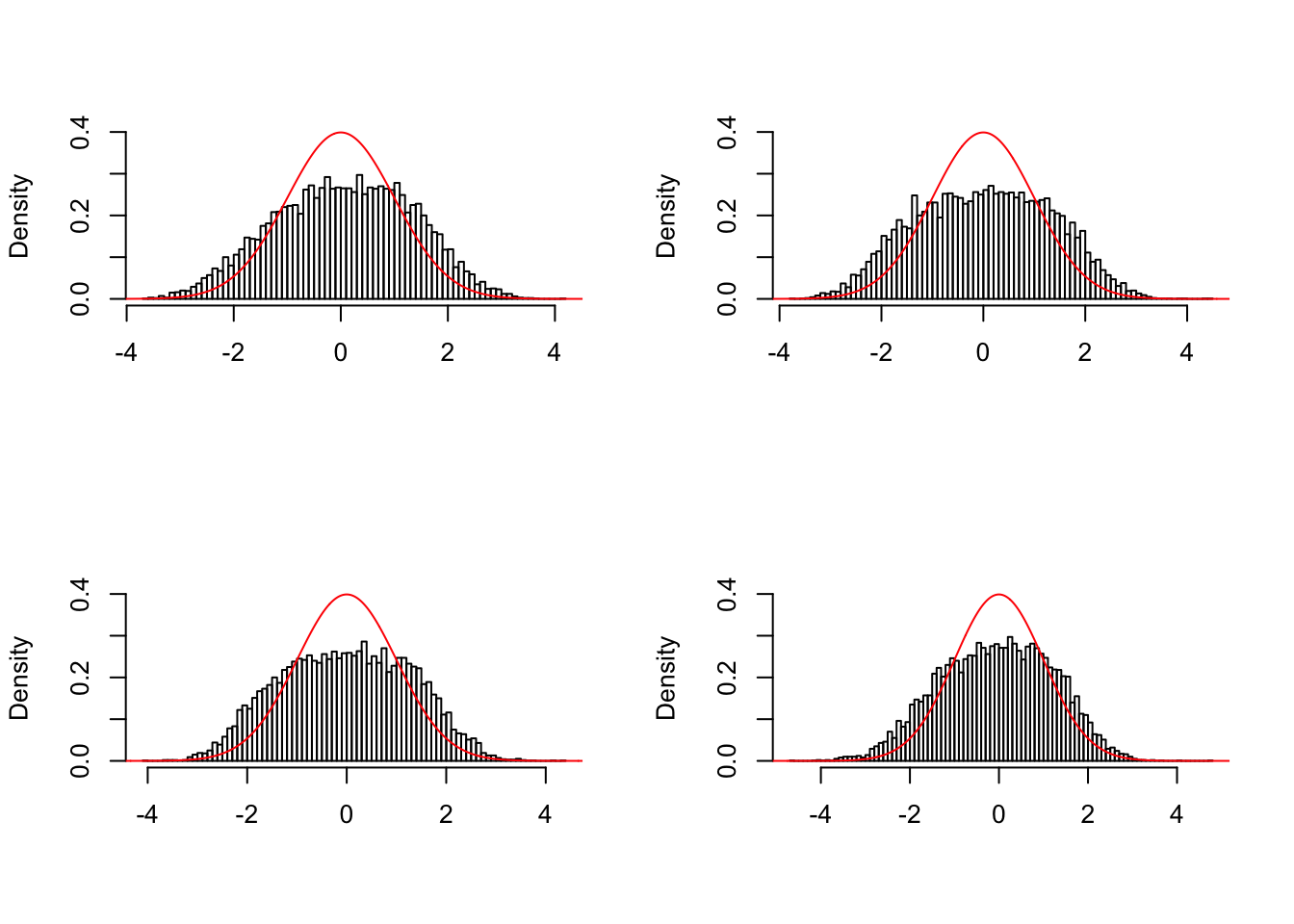
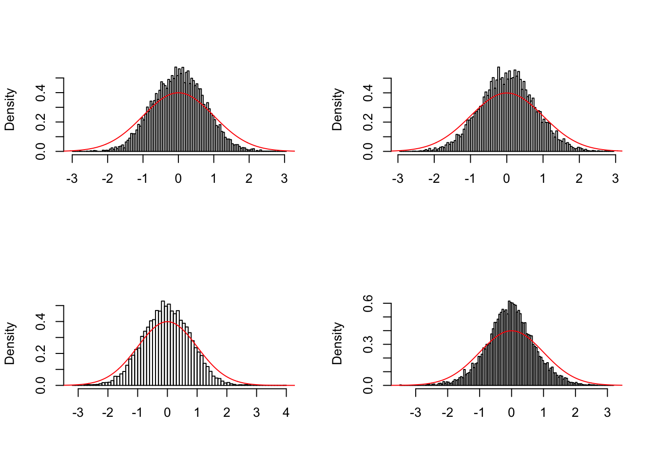
Some examples of inflated correlated null \(z\) scores
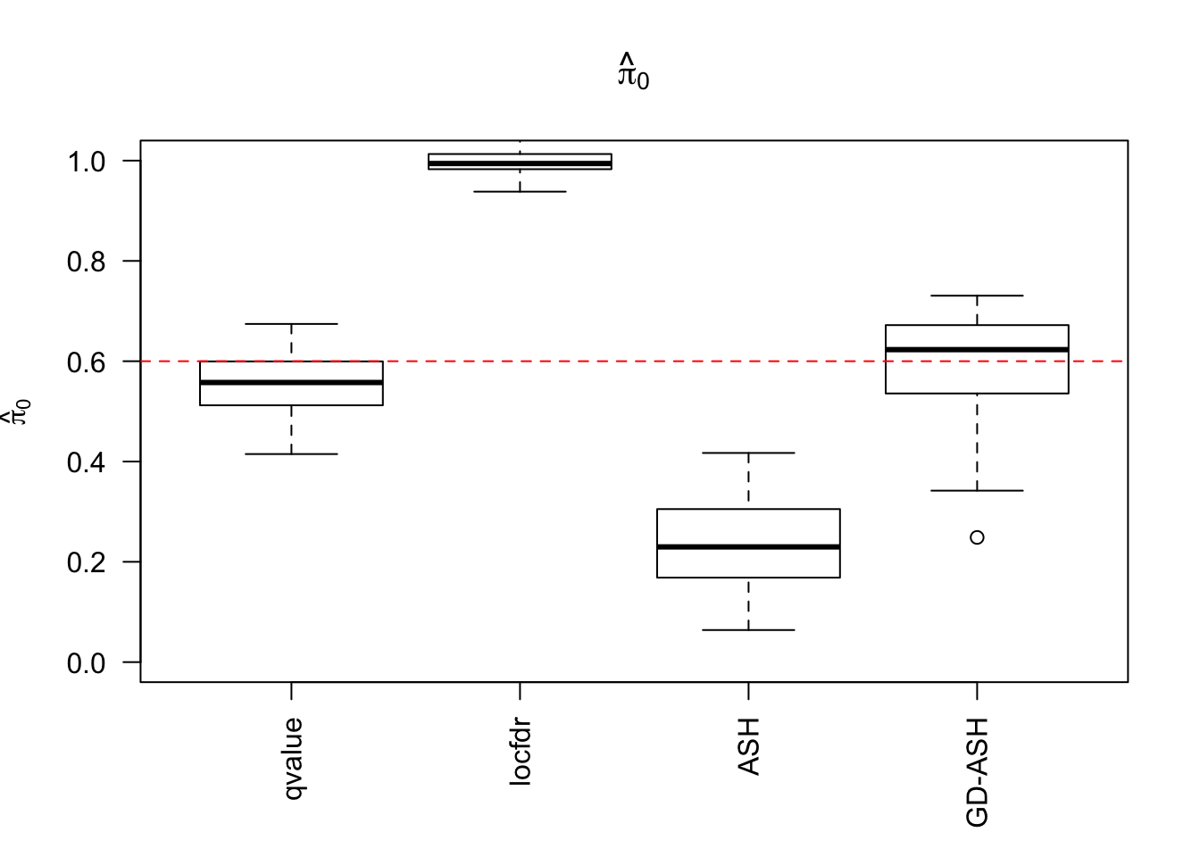
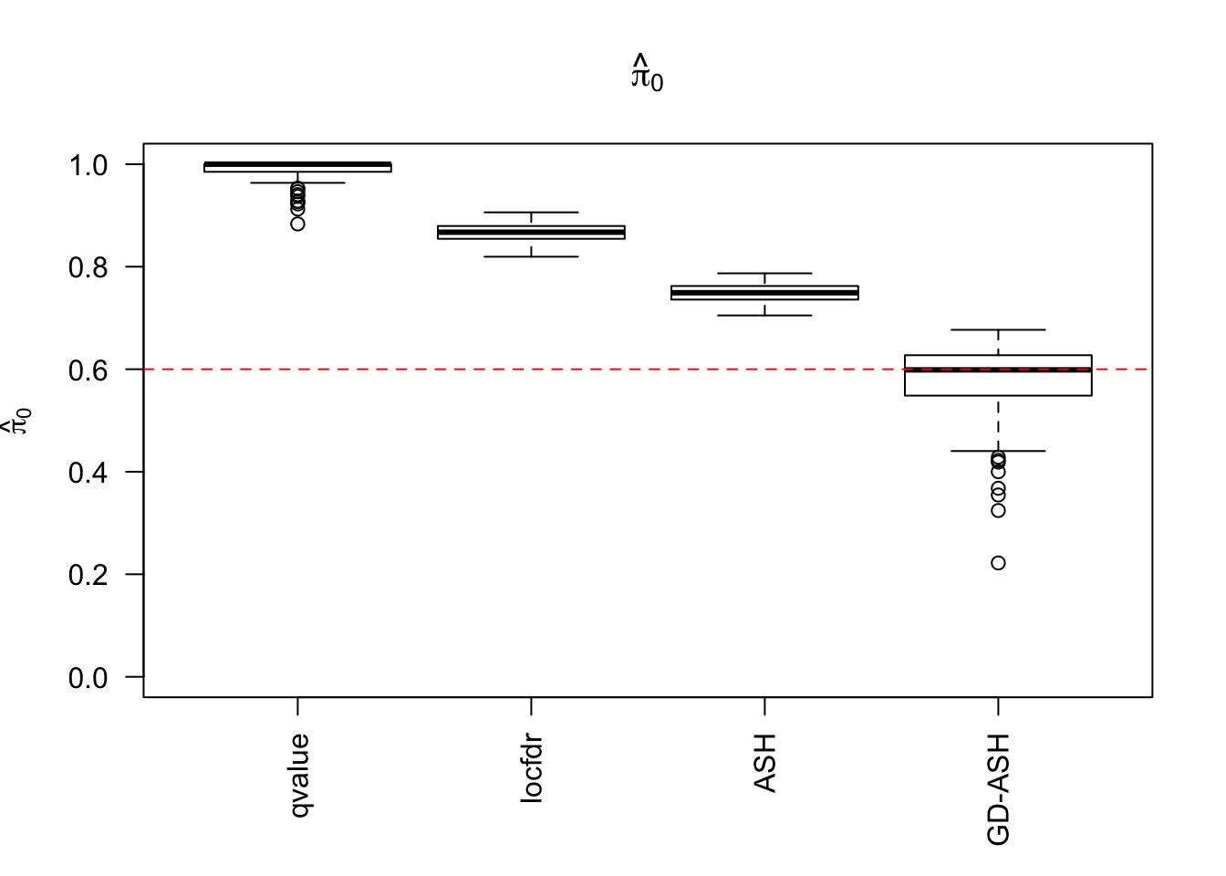
\(\hat \pi_0\)
locfdr overestimates, ASH underestimates, GD-ASH on target, qvalue surprisingly good.
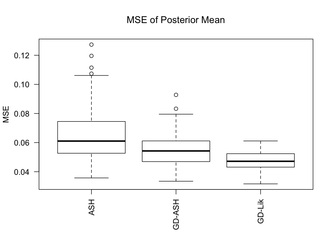
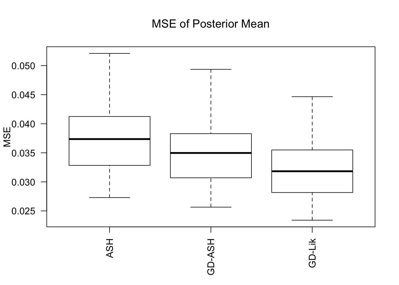
MSE
GD-Lik clearly improves the posterior estimates of GD-ASH.
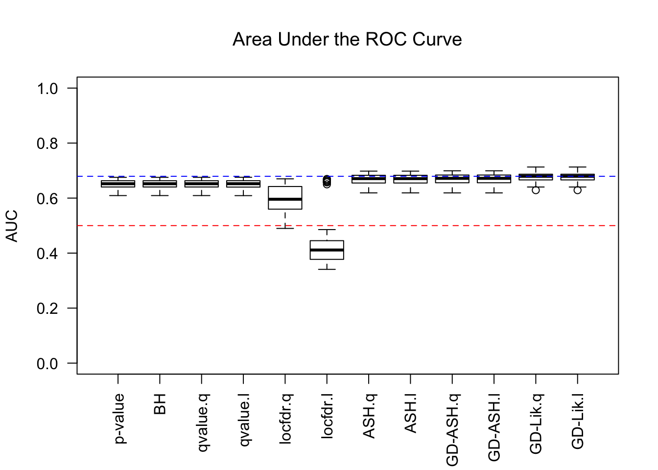
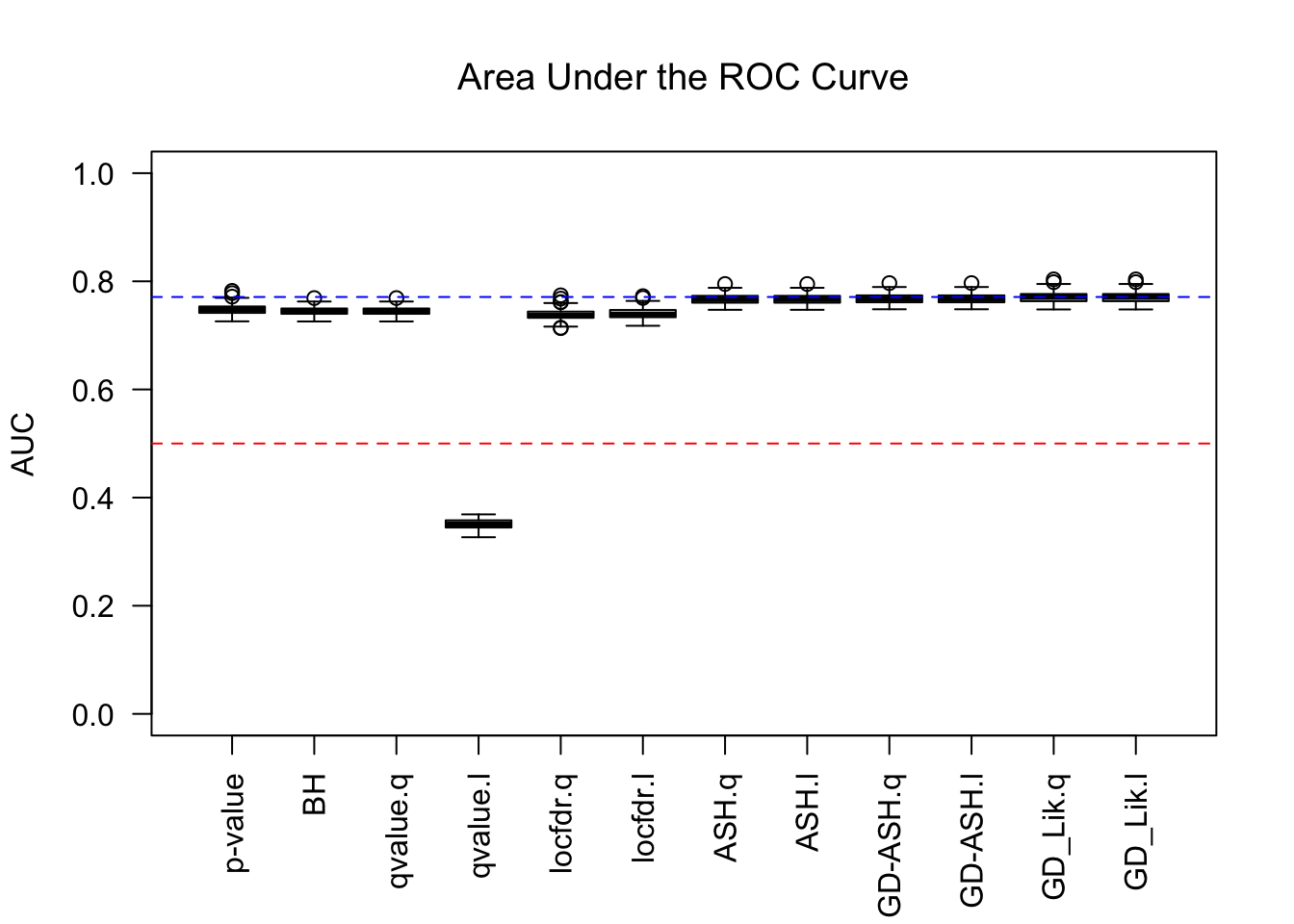
AUC
For almost all methods, .q means using q values, and .l using local FDRs. GD-Lik is the best, yet even the vanilla \(p\) values are not much worse. It indicates that all the methods based on summary statistics indeed make few changes to the order of original \(p\) values. Worth noting is that locfdr doesn’t perform well, and lfdr’s give a drastically different result than q values do, probably due to some artifacts like ties.
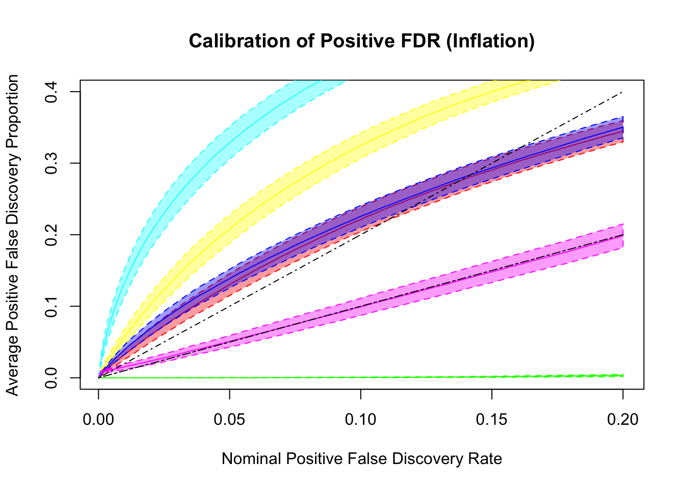
q values and positive FDR (pFDR) calibration
Dashed lines are \(y = x\) and \(y = 2x\). ASH and qvalue are too liberal, and locfdr is too conservative. GD-ASH and BH give very similar results and not far off. BH’s calibrates pFDR relatively well, even though it’s only guaranteed to control FDR under independence. GD-Lik calibrates pFDR almost precisely.
Model and data generation
\[ \begin{array}{l} \hat\beta_j = \beta_j + \sigma_j z_j \\ z_j \sim N(0, 1), \text{ correlated, simulated from real data}\\ \sigma_j : \text{ heteroskedastic, simulated from real data}\\ \beta_j \sim 0.6\delta_0 + 0.3N(0, \sigma^2) + 0.1N\left(0, \left(2\sigma\right)^2\right) \end{array} \]
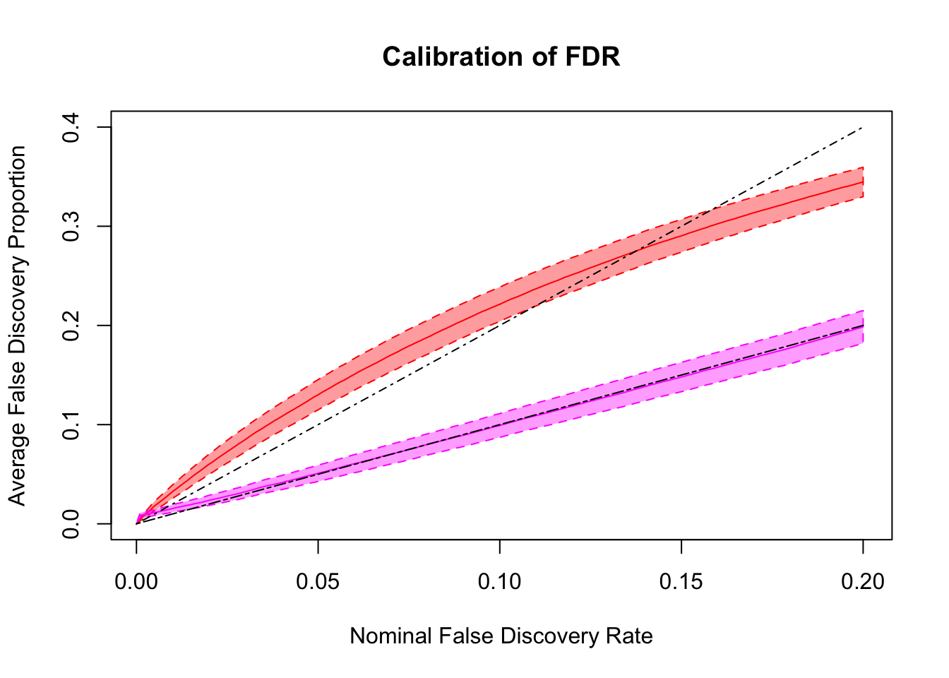
FDR calibration

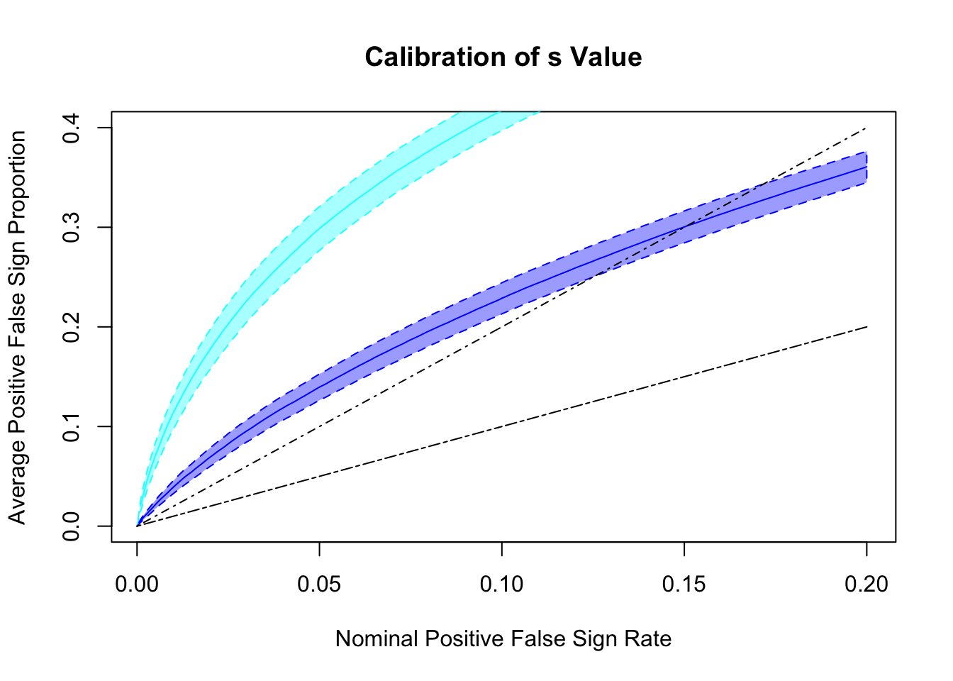
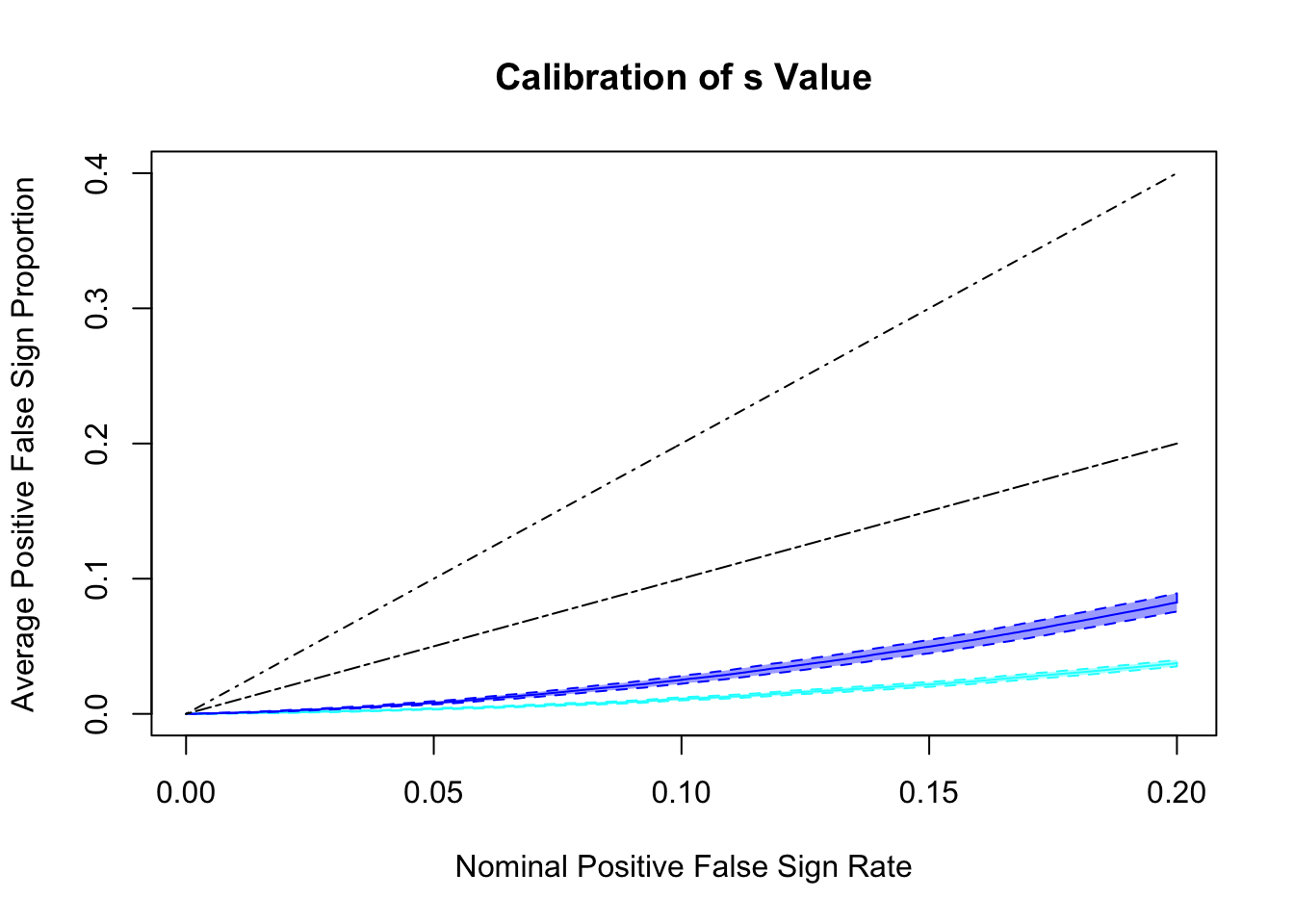
s values and positive FSR (pFSR) calibration
Both ASH and GD-ASH are too liberal, although GD-ASH is not too far off.
Deflation data sets
Some examples of deflated correlated null \(z\) scores
\(\hat \pi_0\)
Almost all methods except GD-ASH overestimate as expected. GD-ASH occasionally severely underestimates as seen before.
MSE
GD-Lik does better than ASH and GD-ASH but not as significantly as in the inflation case.
AUC
Similar story as in the inflation case, although this time qvalue’s lfdr behaves weirdly.
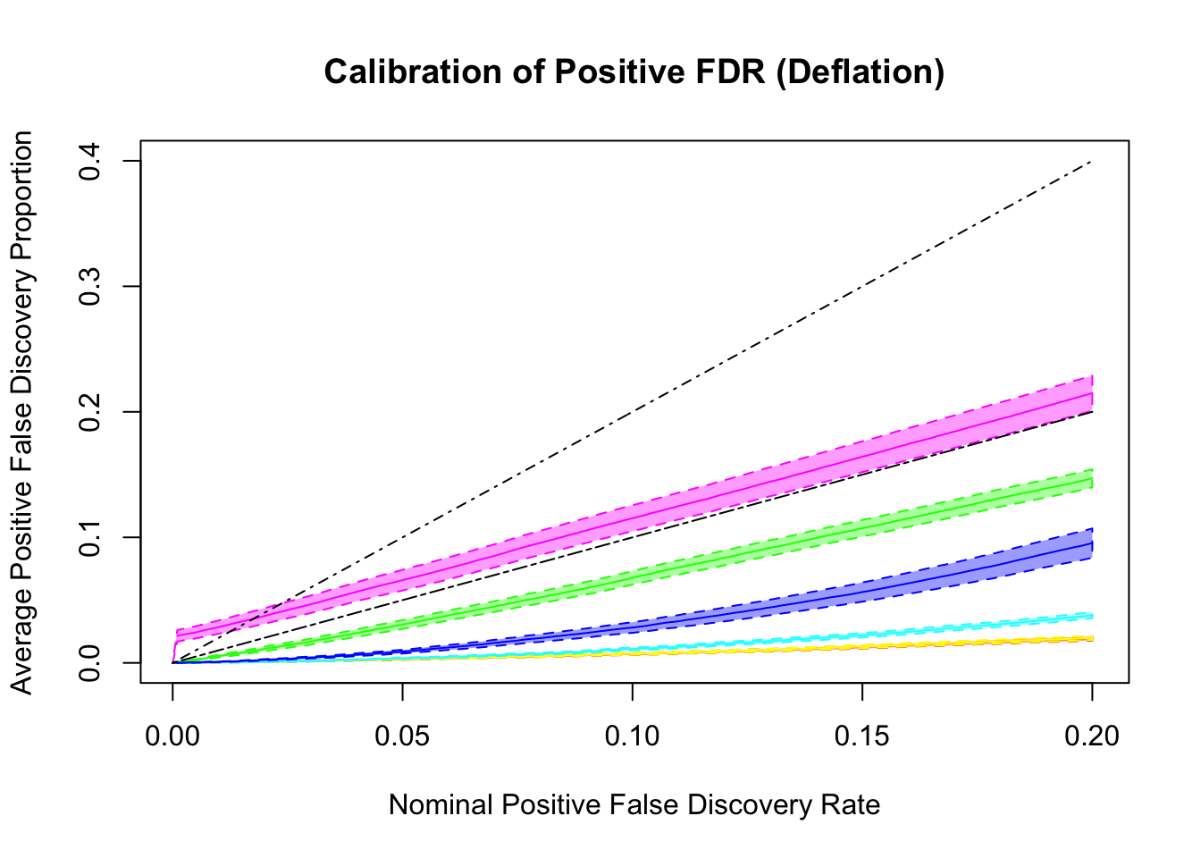
q values and positive FDR (pFDR) calibration
Essentially all methods successfully control pFDR. GD-Lik looks good although off a little. qvalue is the most conservative, followed by ASH, GD-ASH, and locfdr.

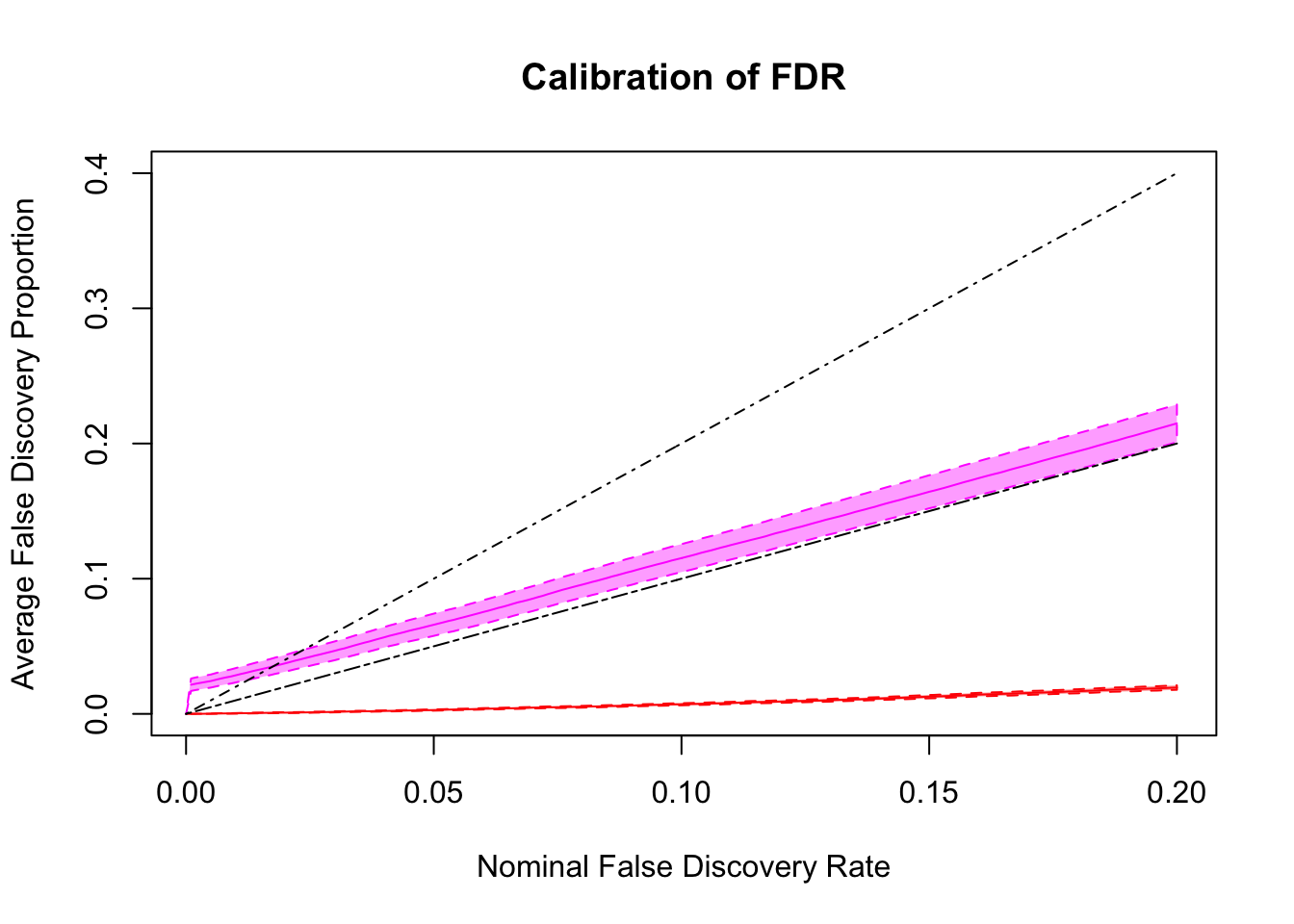
FDR calibration
s values and positive FSR (pFSR) calibration
Both ASH and GD-ASH seem too conservative, although GD-ASH is more powerful.

Remarks
- Would be nice to come up with a way to calculate
lfsrinGD-Lik. - Many methods are too liberal for inflation cases and too conservative for deflation cases, showing a lack of robustness against correlation. Although, on average they probably seem about right.
Session information
sessionInfo()R version 3.4.3 (2017-11-30)
Platform: x86_64-apple-darwin15.6.0 (64-bit)
Running under: macOS High Sierra 10.13.2
Matrix products: default
BLAS: /Library/Frameworks/R.framework/Versions/3.4/Resources/lib/libRblas.0.dylib
LAPACK: /Library/Frameworks/R.framework/Versions/3.4/Resources/lib/libRlapack.dylib
locale:
[1] en_US.UTF-8/en_US.UTF-8/en_US.UTF-8/C/en_US.UTF-8/en_US.UTF-8
attached base packages:
[1] stats graphics grDevices utils datasets methods base
other attached packages:
[1] ashr_2.2-2 Rmosek_8.0.69 PolynomF_1.0-1 CVXR_0.94-4
[5] REBayes_1.2 Matrix_1.2-12 SQUAREM_2017.10-1 EQL_1.0-0
[9] ttutils_1.0-1
loaded via a namespace (and not attached):
[1] gmp_0.5-13.1 Rcpp_0.12.14 compiler_3.4.3
[4] git2r_0.20.0 R.methodsS3_1.7.1 R.utils_2.6.0
[7] iterators_1.0.9 tools_3.4.3 digest_0.6.13
[10] bit_1.1-12 evaluate_0.10.1 lattice_0.20-35
[13] foreach_1.4.4 yaml_2.1.16 parallel_3.4.3
[16] Rmpfr_0.6-1 ECOSolveR_0.3-2 stringr_1.2.0
[19] knitr_1.17 rprojroot_1.3-1 bit64_0.9-7
[22] grid_3.4.3 R6_2.2.2 rmarkdown_1.8
[25] magrittr_1.5 MASS_7.3-47 backports_1.1.2
[28] codetools_0.2-15 htmltools_0.3.6 scs_1.1-1
[31] stringi_1.1.6 doParallel_1.0.11 pscl_1.5.2
[34] truncnorm_1.0-7 R.oo_1.21.0 This R Markdown site was created with workflowr