Marginal Distribution of \(z\) Scores: Alternative
Lei Sun
2017-05-08
Last updated: 2017-12-21
Code version: 6e42447
Introduction
We’ve seen that when generated from the global null, that is, when the cases and controls have no difference, the \(z\) scores’ behavior are what one would expect if simulated from correlated marginally \(N\left(0, 1\right)\) random variables.
But what if the \(z\) scores are not simulated from the global null? Are these \(z\) scores going to behave significantly different from correlated marginally \(N\left(0, 1\right)\) random samples? Let’s take a look at the real data containing true effects.
library(limma)
library(edgeR)
library(qvalue)
library(ashr)

#extract top g genes from G by n matrix X of expression

top_genes_index = function (g, X)
{return(order(rowSums(X), decreasing = TRUE)[1 : g])
}

lcpm = function (r) {
  R = colSums(r)
  t(log2(((t(r) + 0.5) / (R + 1)) * 10^6))
}

# transform counts to z scores
# these z scores are marginally N(0, 1) under null

counts_to_z = function (counts, condition) {
  design = model.matrix(~condition)
  dgecounts = calcNormFactors(DGEList(counts = counts, group = condition))
  v = voom(dgecounts, design, plot = FALSE)
  lim = lmFit(v)
  r.ebayes = eBayes(lim)
  p = r.ebayes$p.value[, 2]
  t = r.ebayes$t[, 2]
  z = sign(t) * qnorm(1 - p/2)
  return (z)
}
Generating non-null \(z\) scores from real data
For convenience and without loss of generality, we are using the liver tissue as an anchor in the simulation, and always choose top expressed genes in livers.
r.liver = read.csv("../data/liver.csv")
r.liver = r.liver[, -(1 : 2)] # remove gene name and description
Y = lcpm(r.liver)
G = 1e4
subset = top_genes_index(G, Y)
r.liver = r.liver[subset, ]
Liver vs Heart
tissue = "heart"
r = read.csv(paste0("../data/", tissue, ".csv"))
r = r[, -(1 : 2)] # remove gene name and description
## choose top expressed genes in liver
r = r[subset, ]
set.seed(777)
m = 1e3
n = 5
z.list = list()
condition = c(rep(0, n), rep(1, n))
for (i in 1 : m) {
counts = cbind(r.liver[, sample(1 : ncol(r.liver), n)],
r[, sample(1 : ncol(r), n)])
z.list[[i]] = counts_to_z(counts, condition)
}z.mat = matrix(unlist(z.list), nrow = m, byrow = TRUE)
saveRDS(z.mat, "../output/z_5liver_5heart_777.rds")Liver vs Muscle
tissue = "muscle"
r = read.csv(paste0("../data/", tissue, ".csv"))
r = r[, -(1 : 2)] # remove gene name and description
## choose top expressed genes in liver
r = r[subset, ]
set.seed(777)
m = 1e3
n = 5
z.list = list()
condition = c(rep(0, n), rep(1, n))
for (i in 1 : m) {
counts = cbind(r.liver[, sample(1 : ncol(r.liver), n)],
r[, sample(1 : ncol(r), n)])
z.list[[i]] = counts_to_z(counts, condition)
}z.mat = matrix(unlist(z.list), nrow = m, byrow = TRUE)
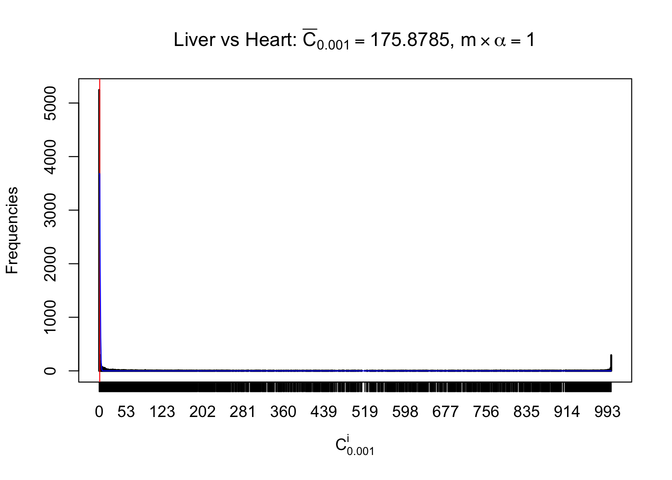
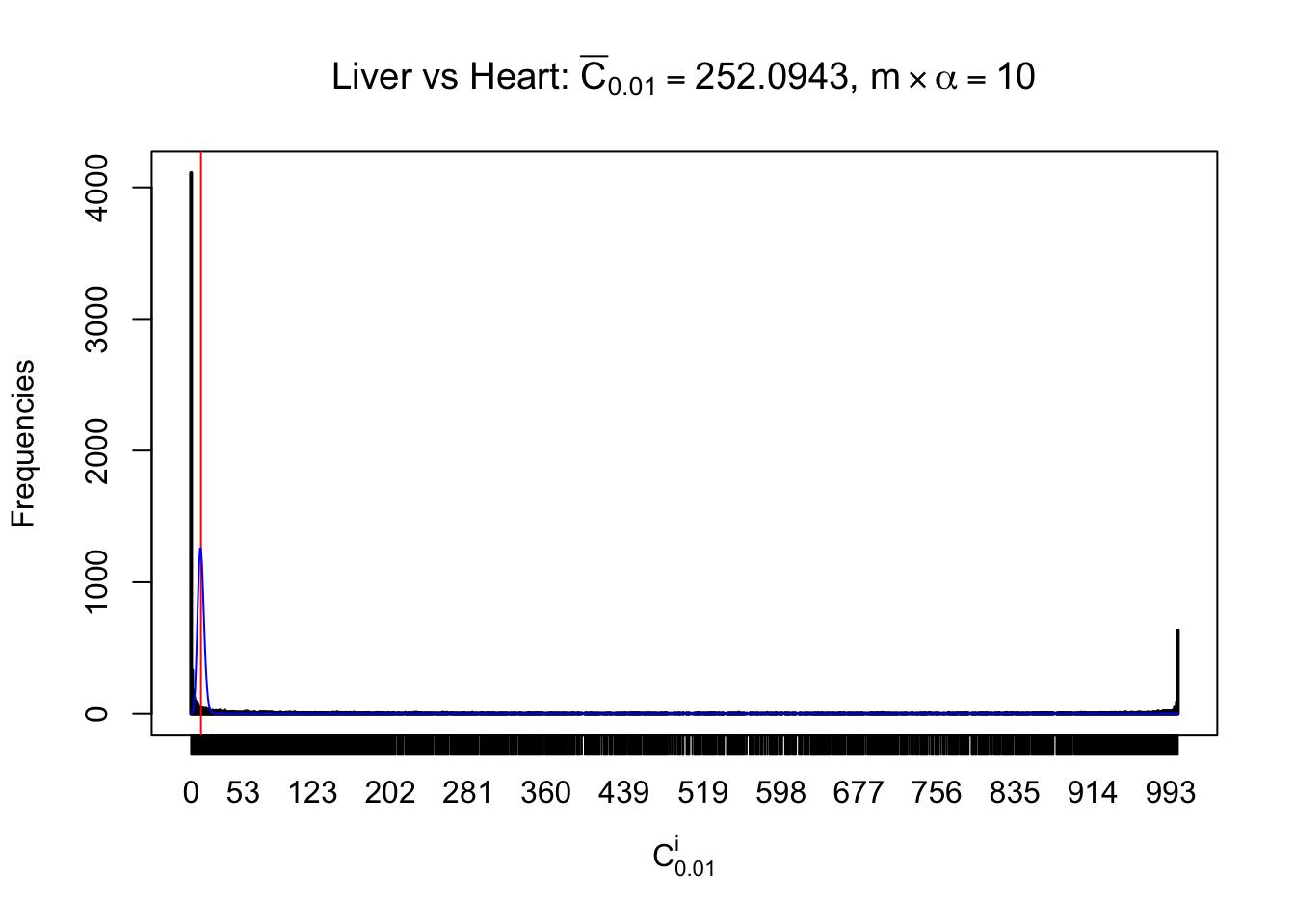
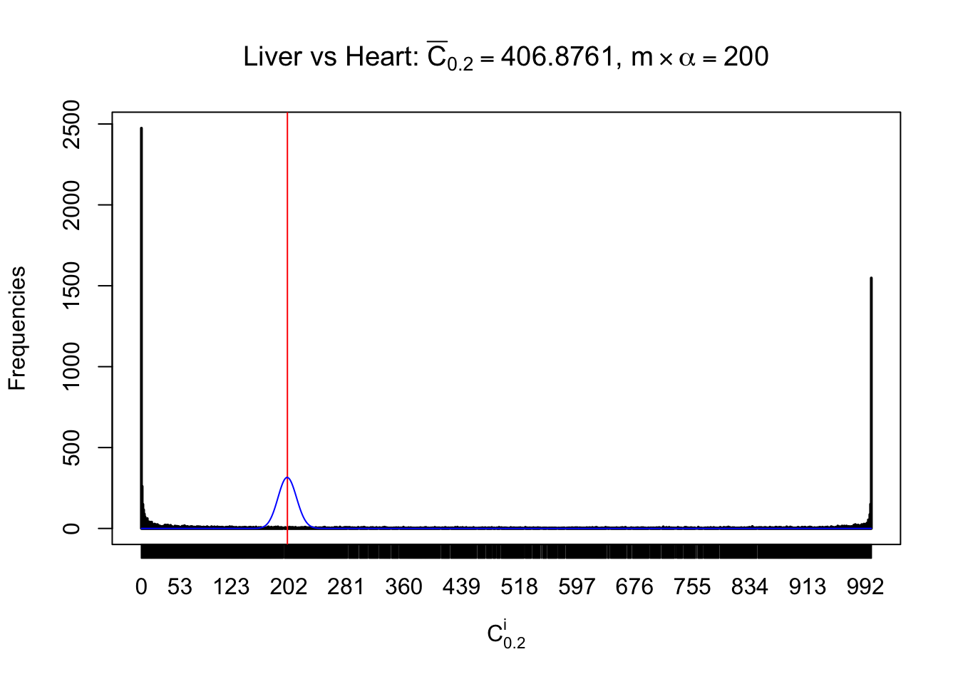
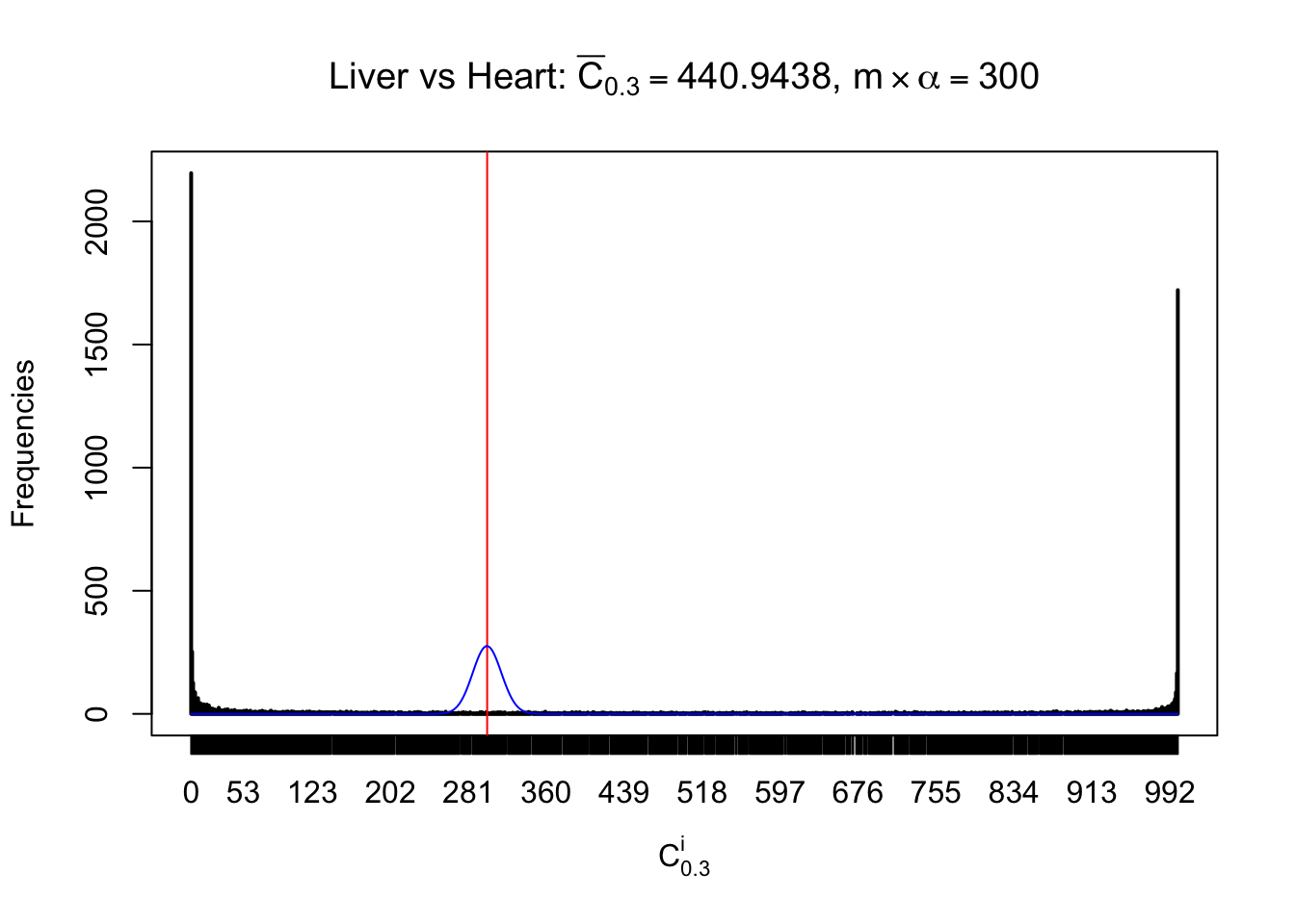
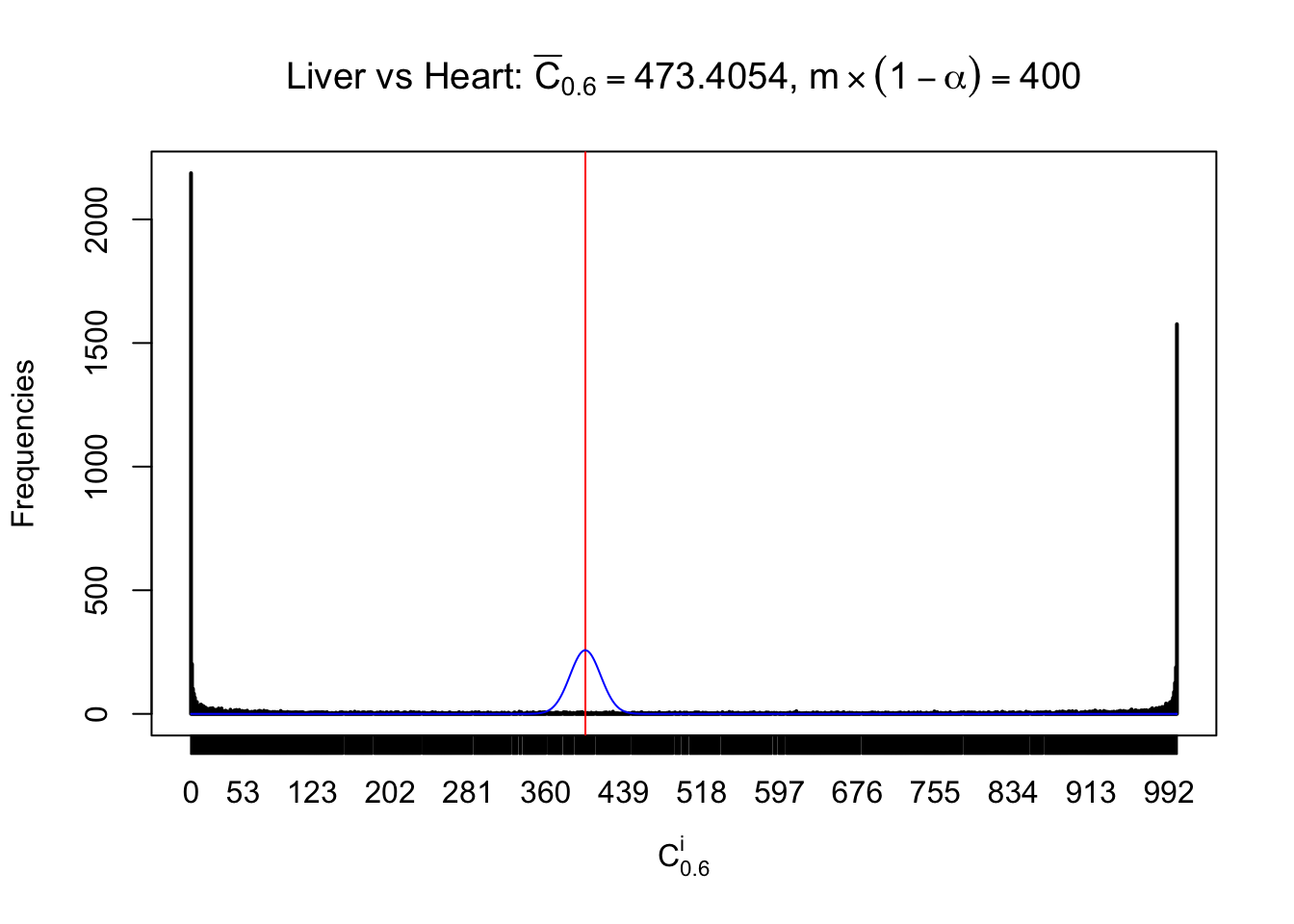
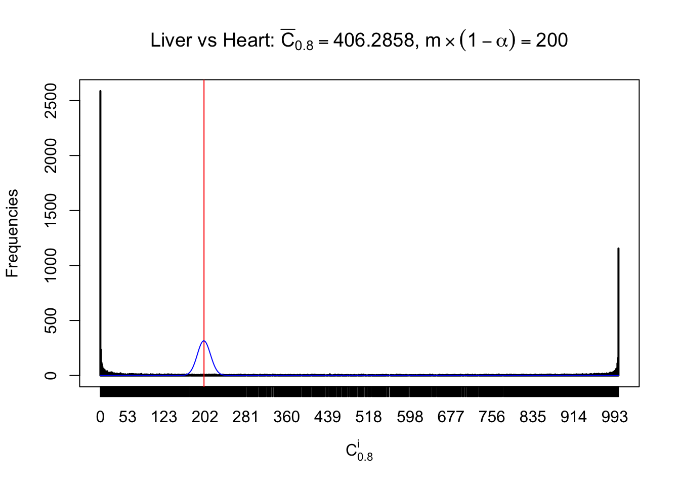
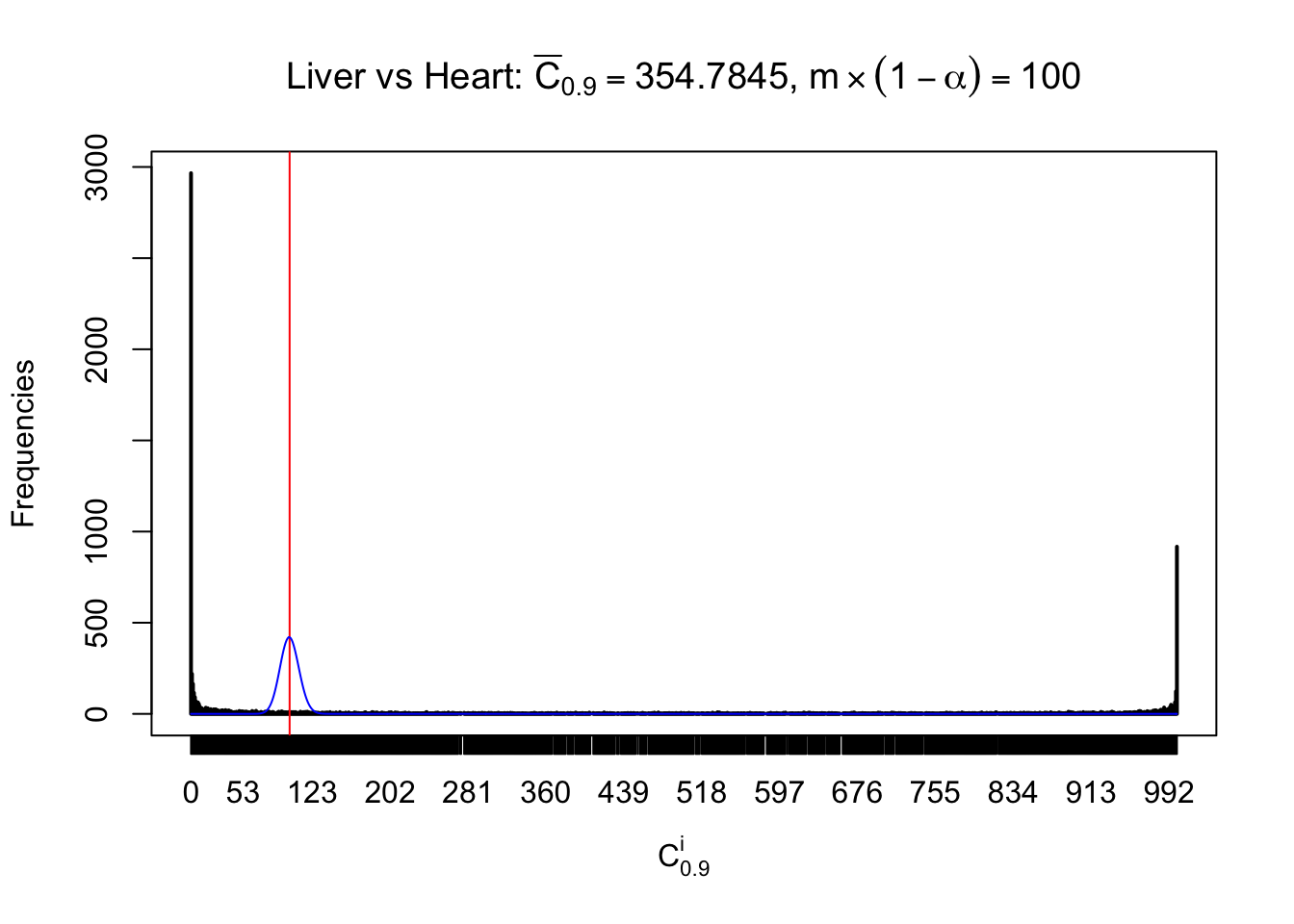
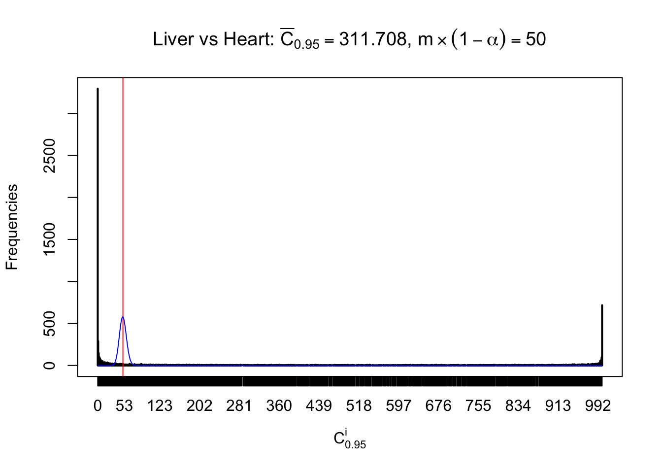
saveRDS(z.mat, "../output/z_5liver_5muscle_777.rds")Liver vs Heart
z.heart = readRDS("../output/z_5liver_5heart_777.rds")
n = ncol(z.heart)
m = nrow(z.heart)
Row-wise
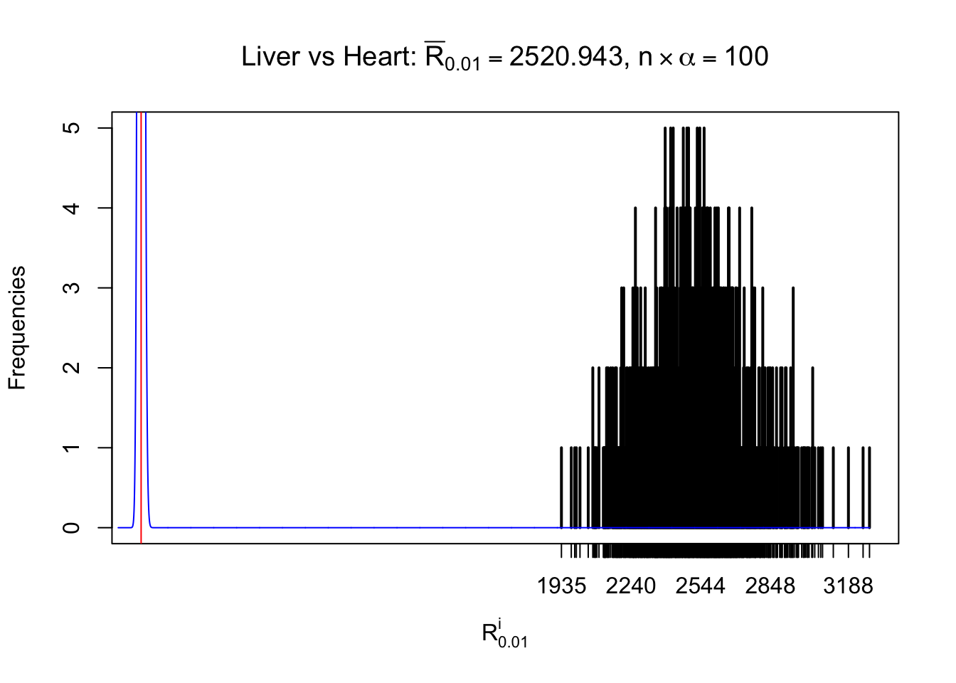
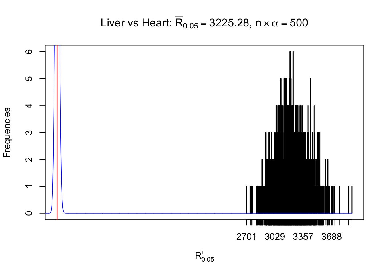
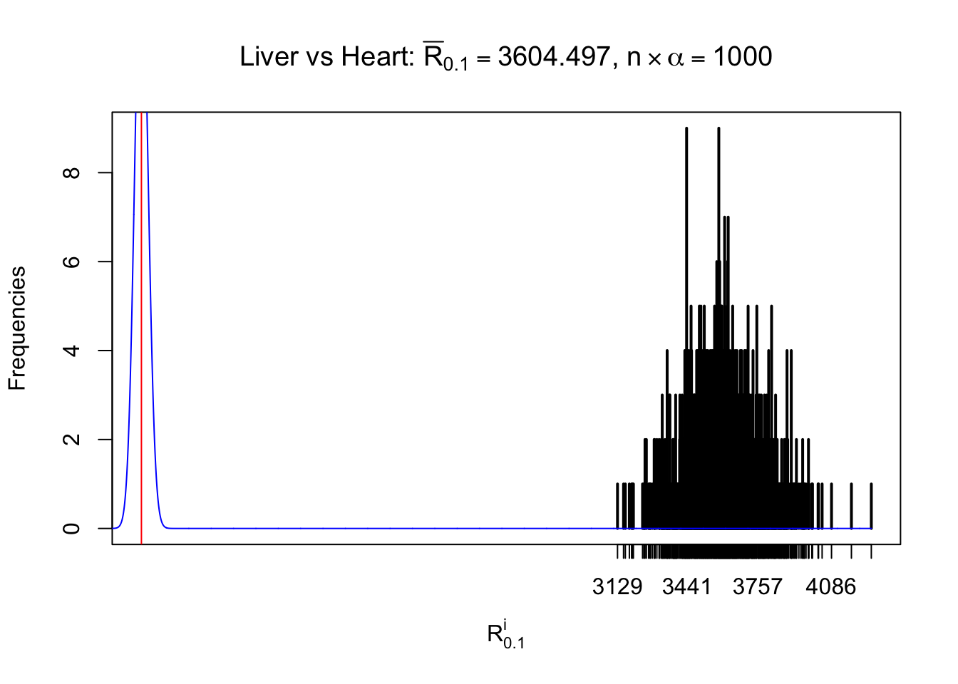
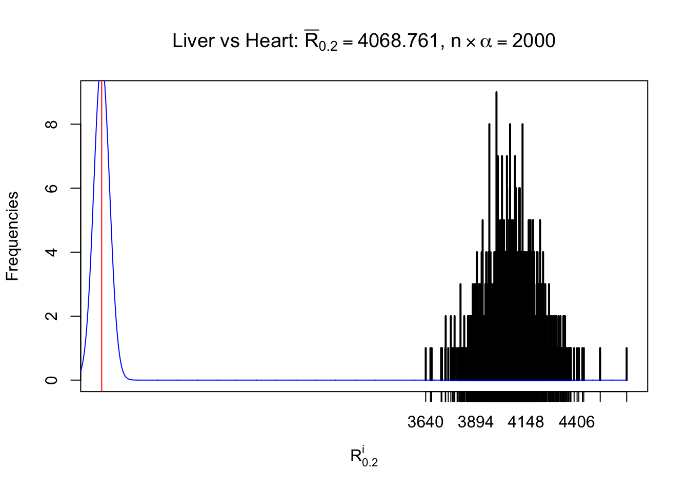
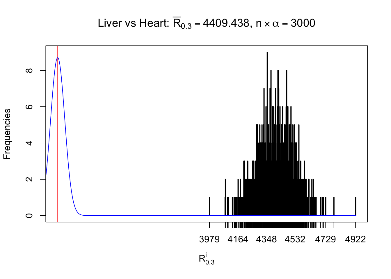
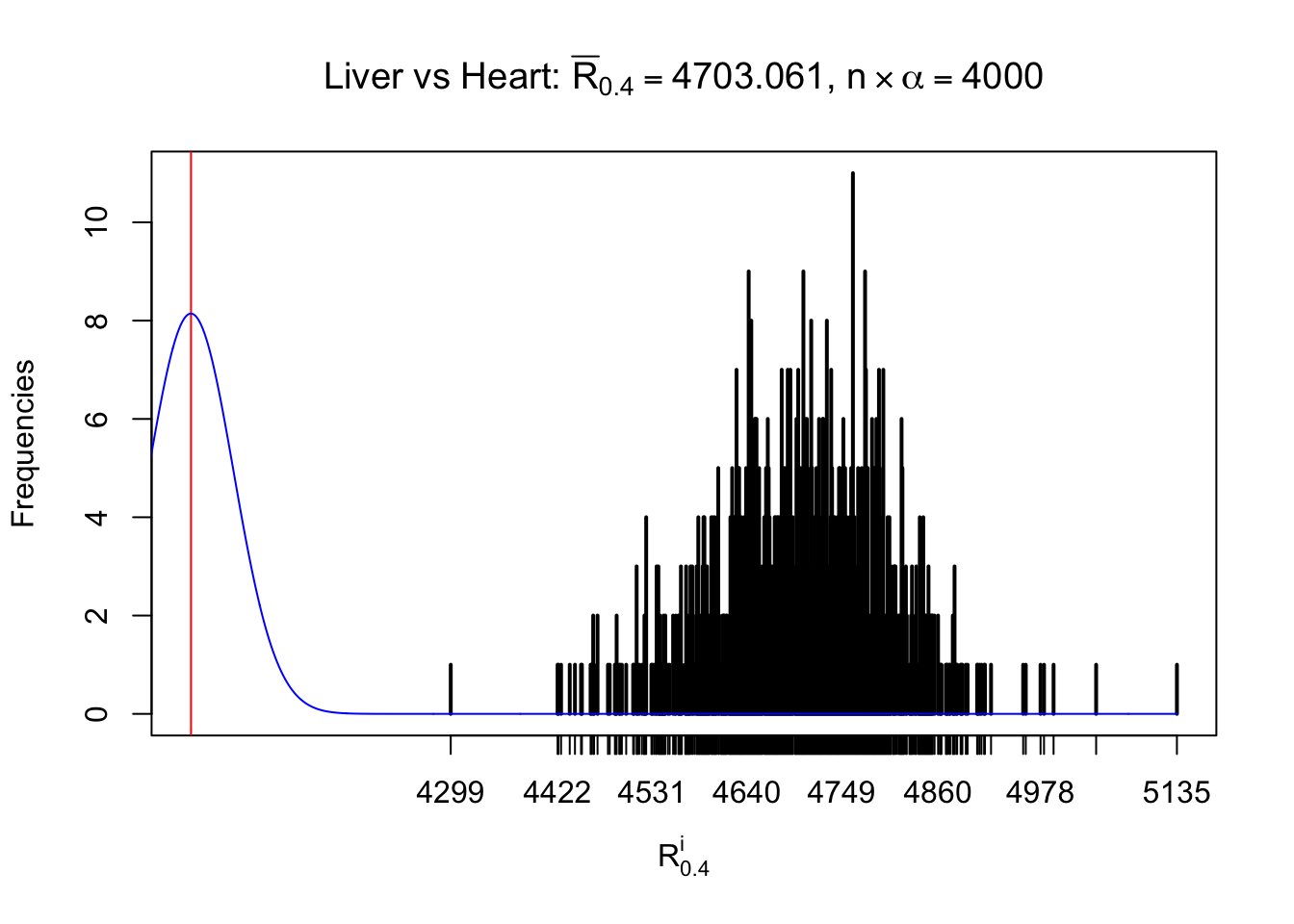
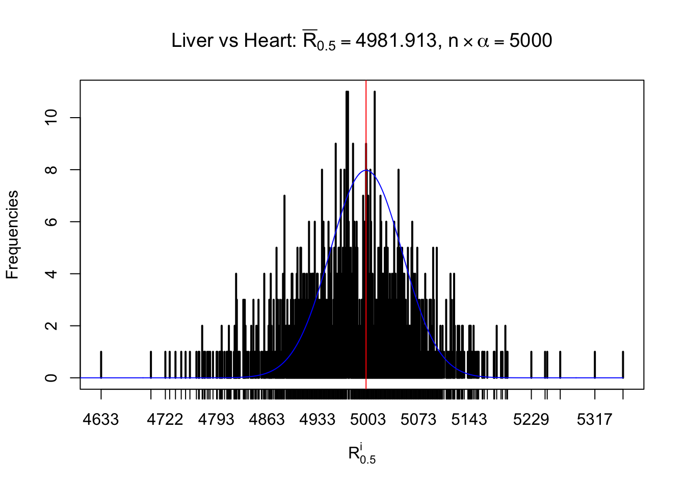
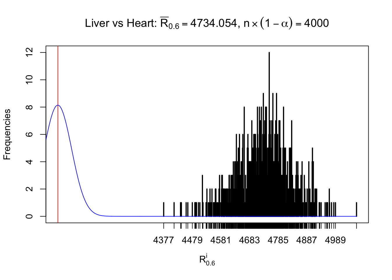
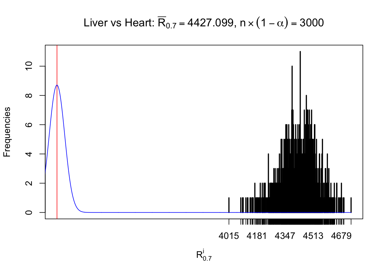

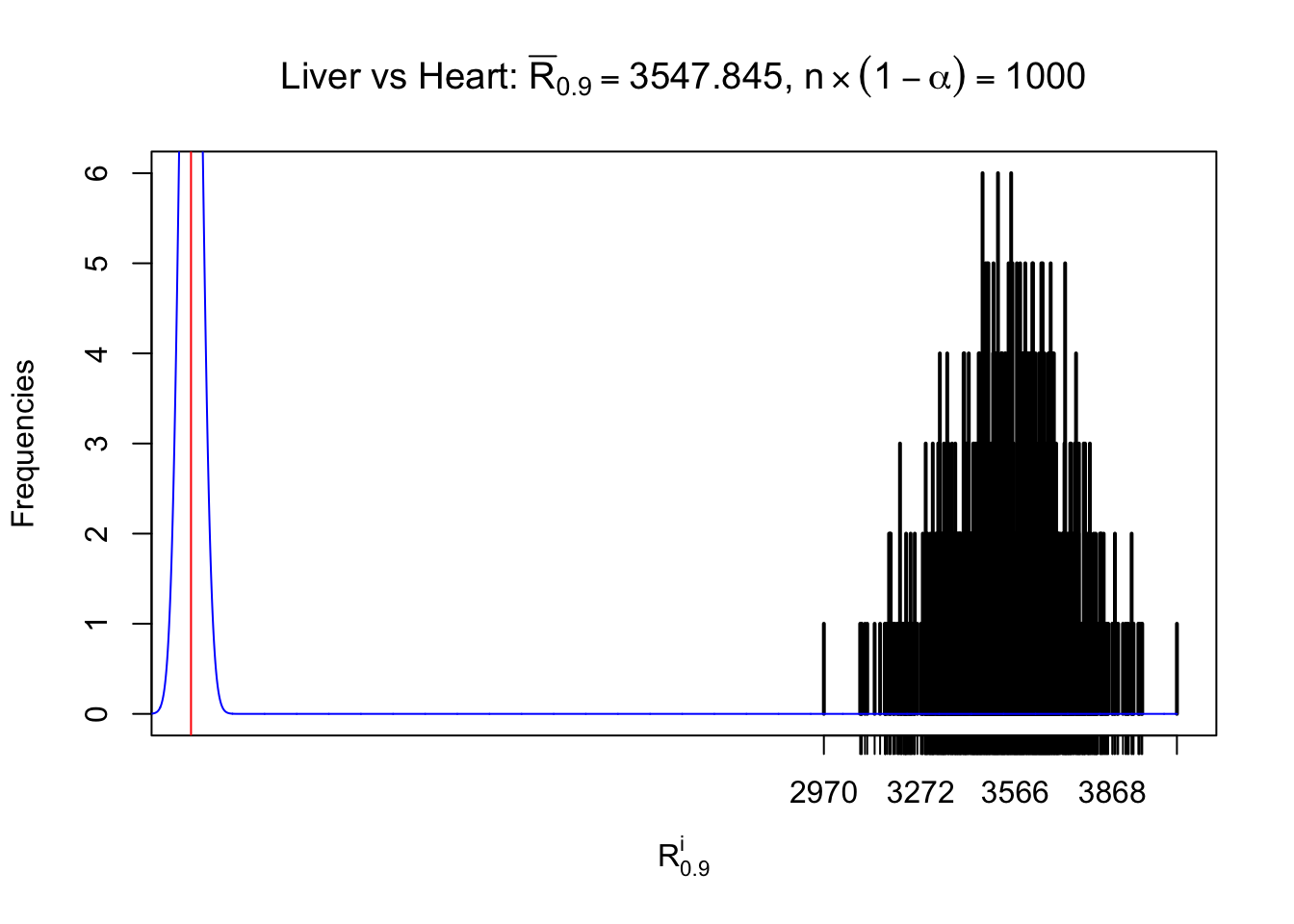
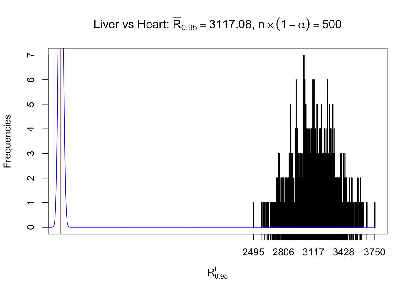
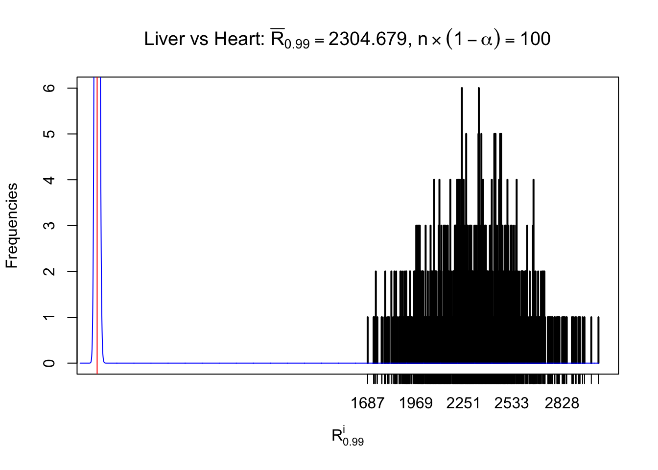
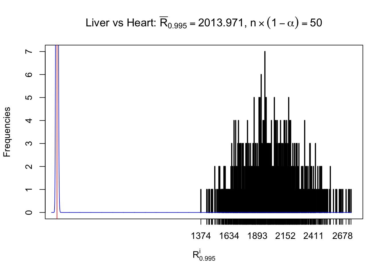
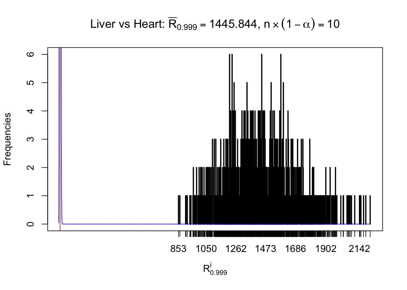
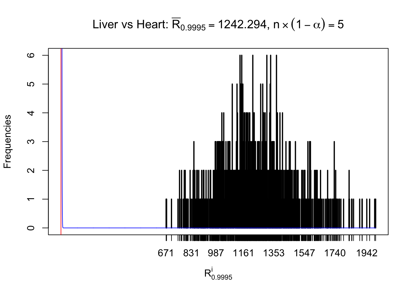
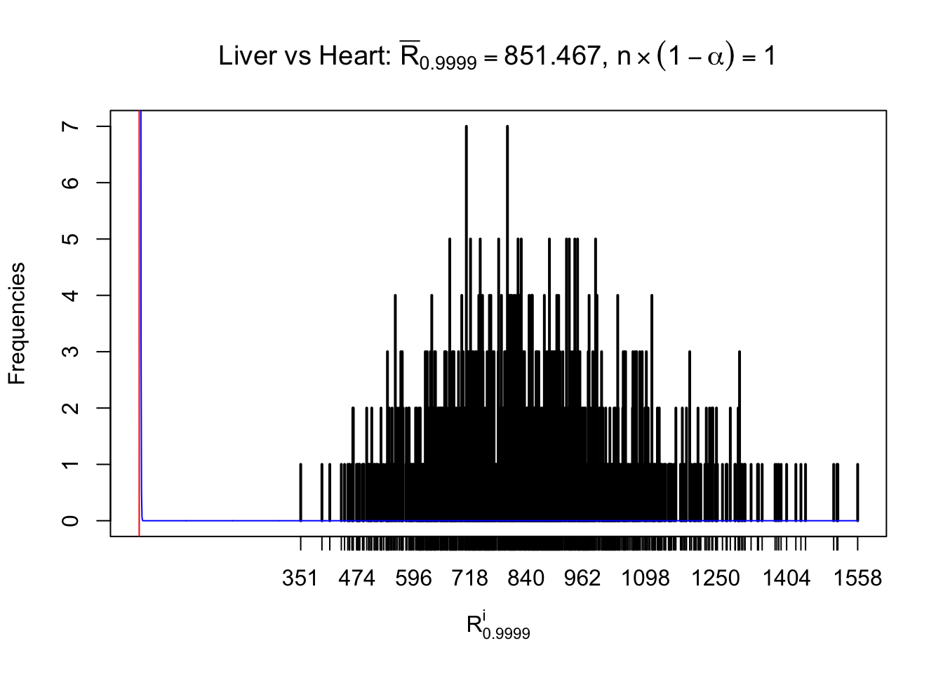
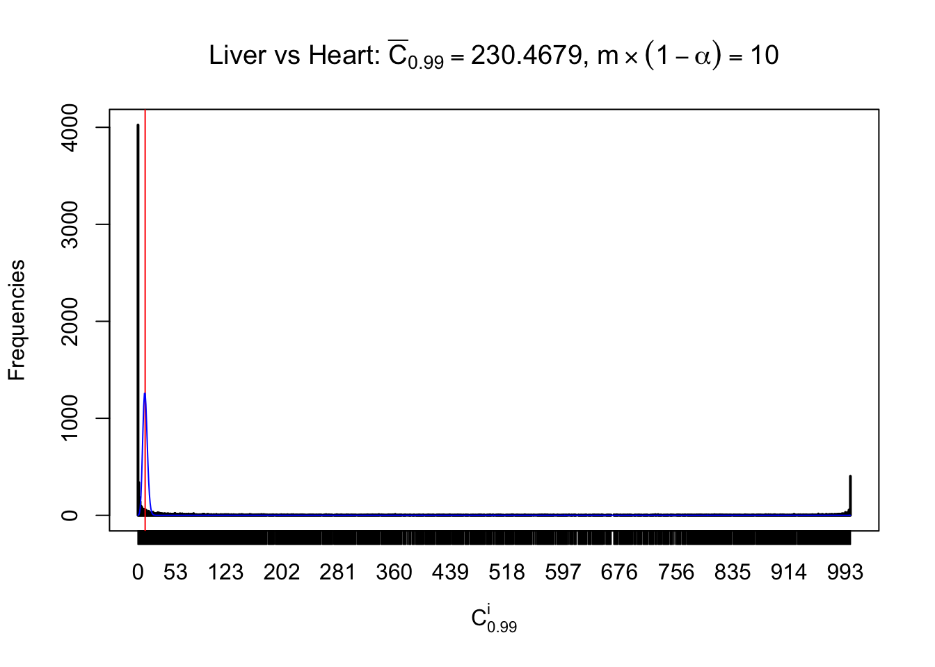
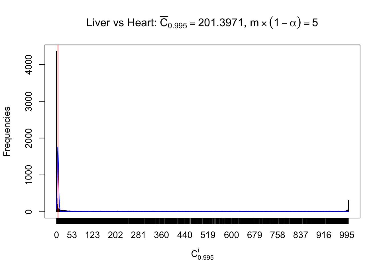
Column-wise


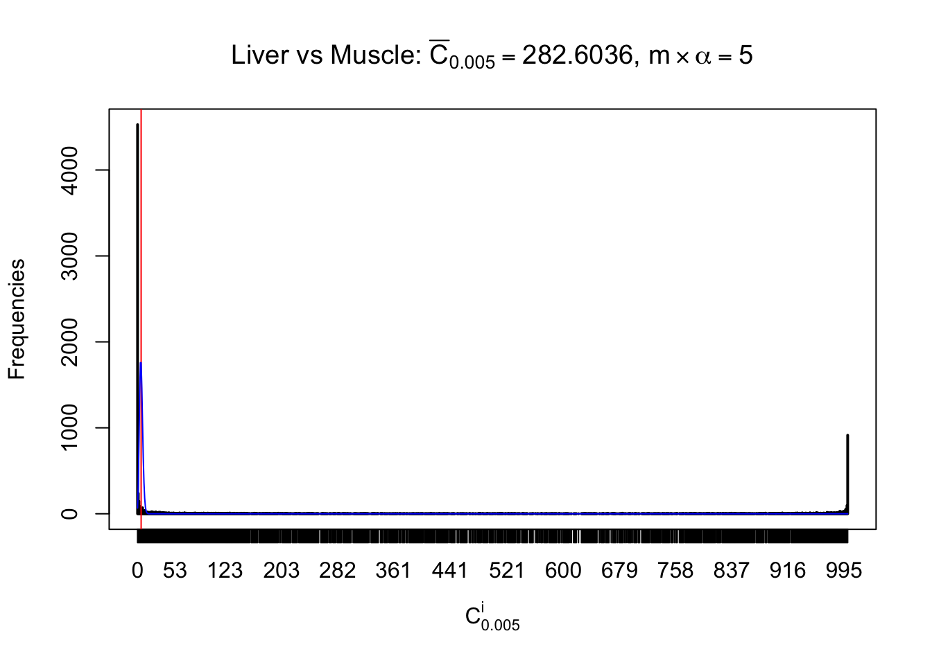
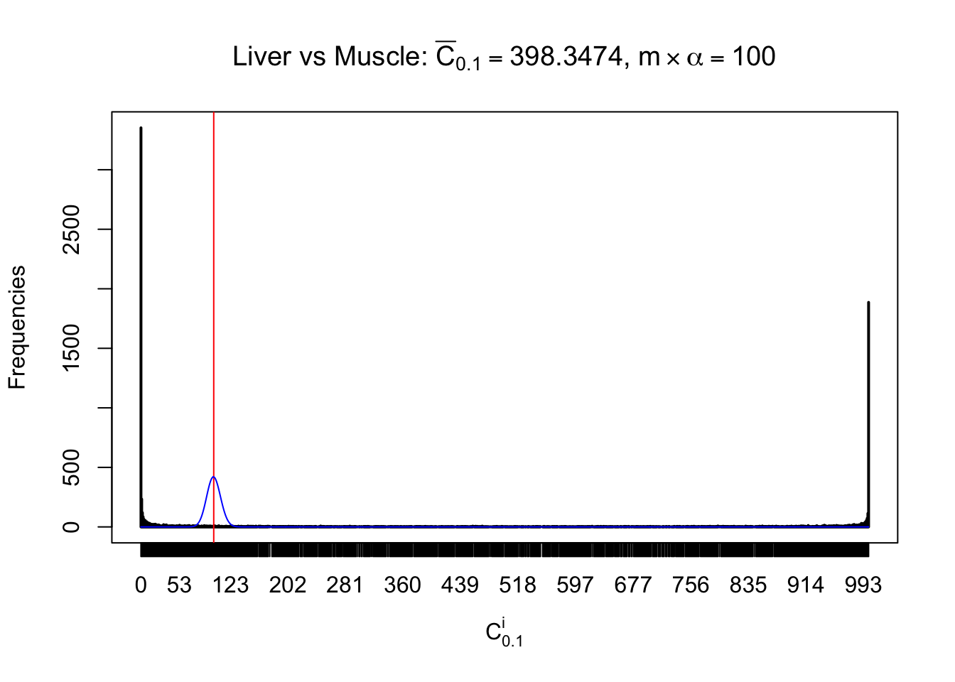
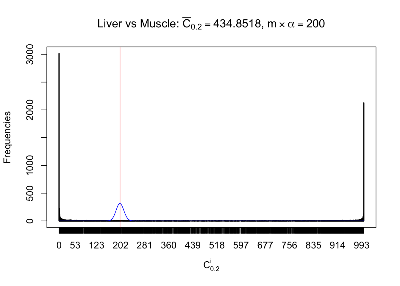
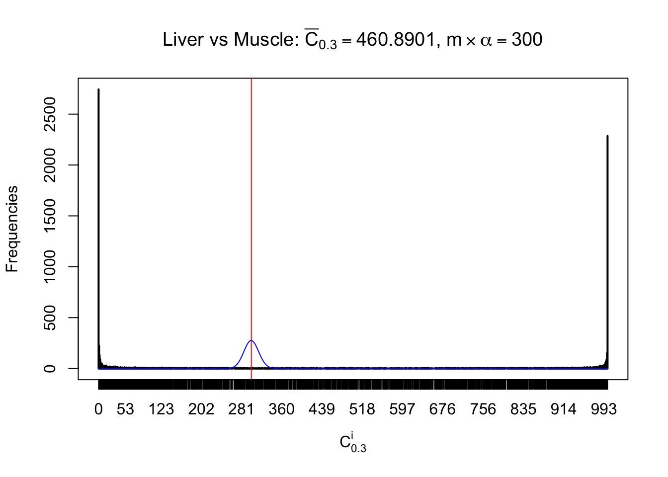
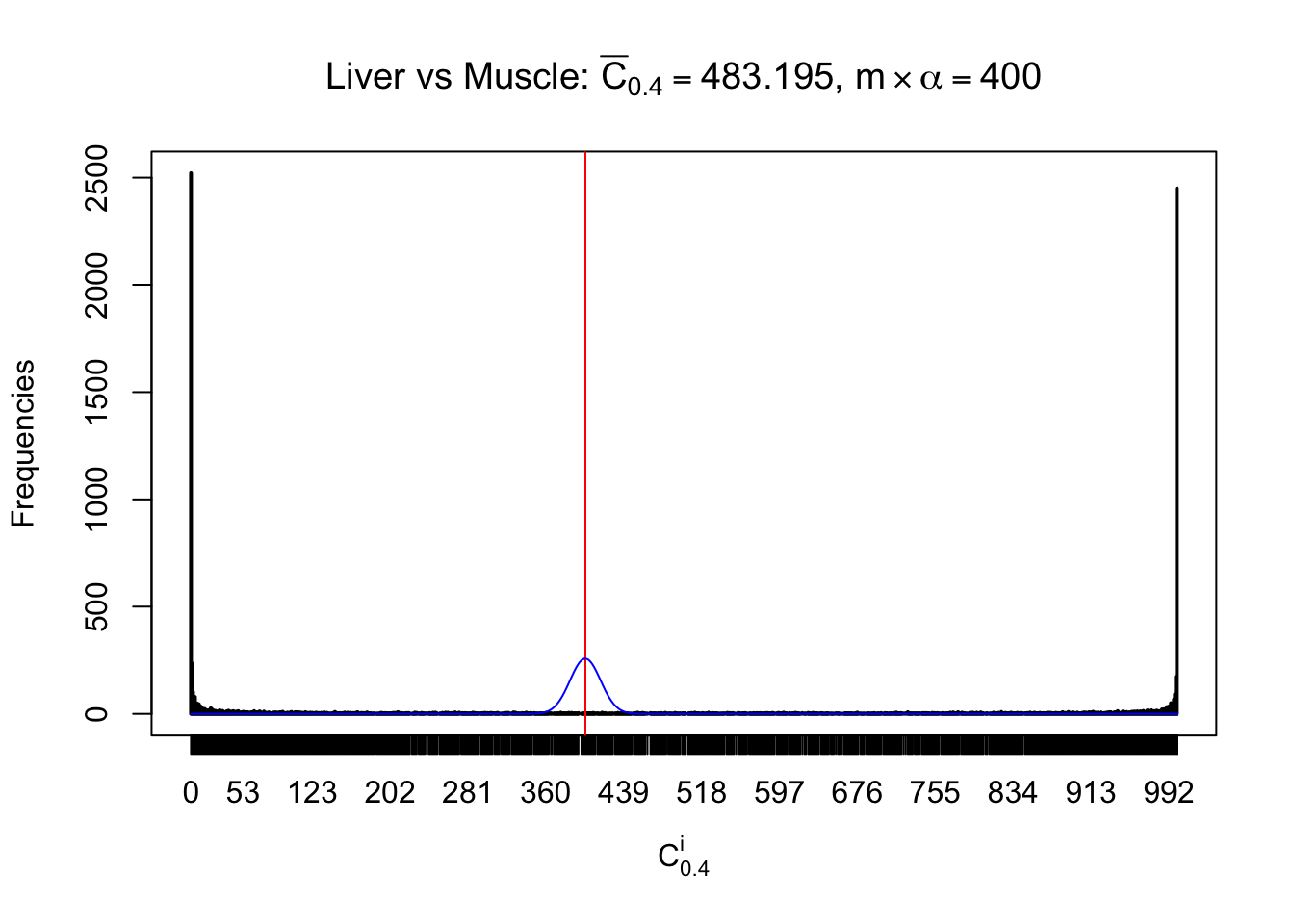
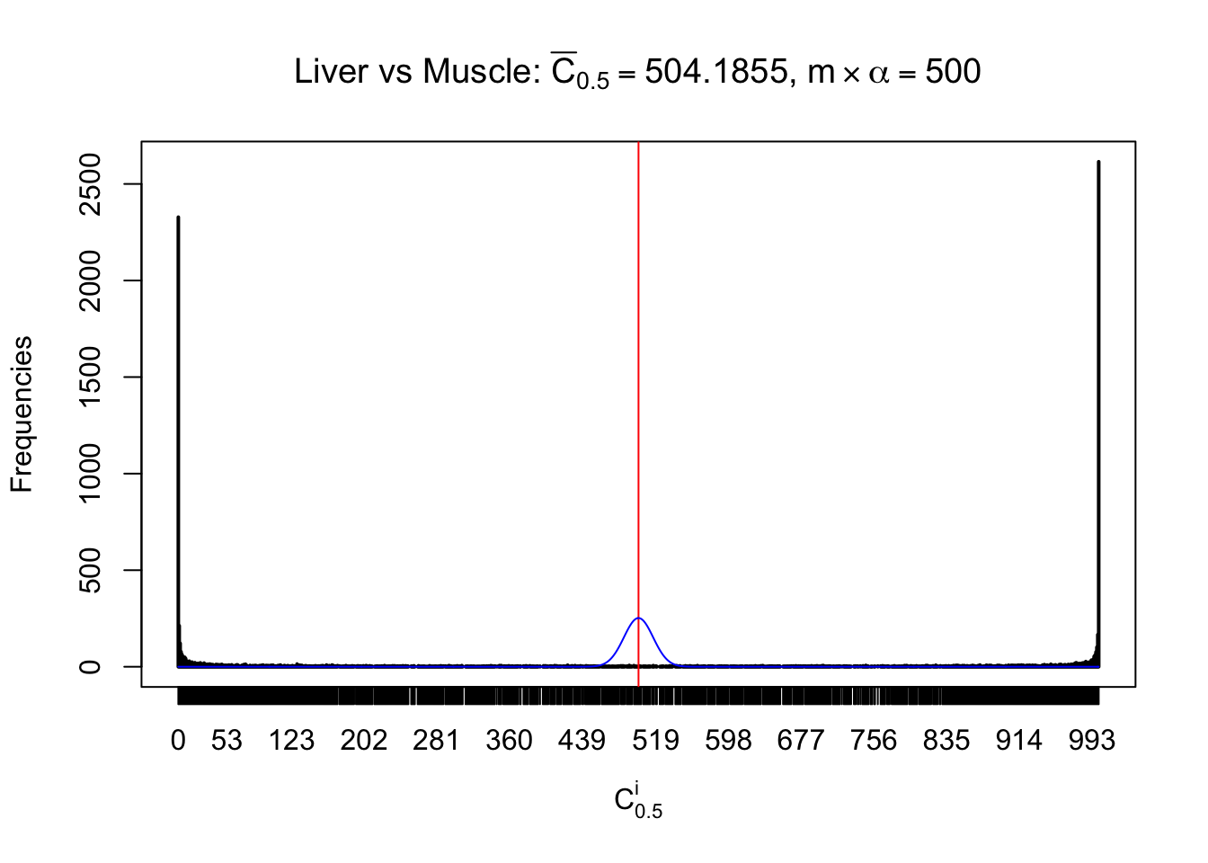
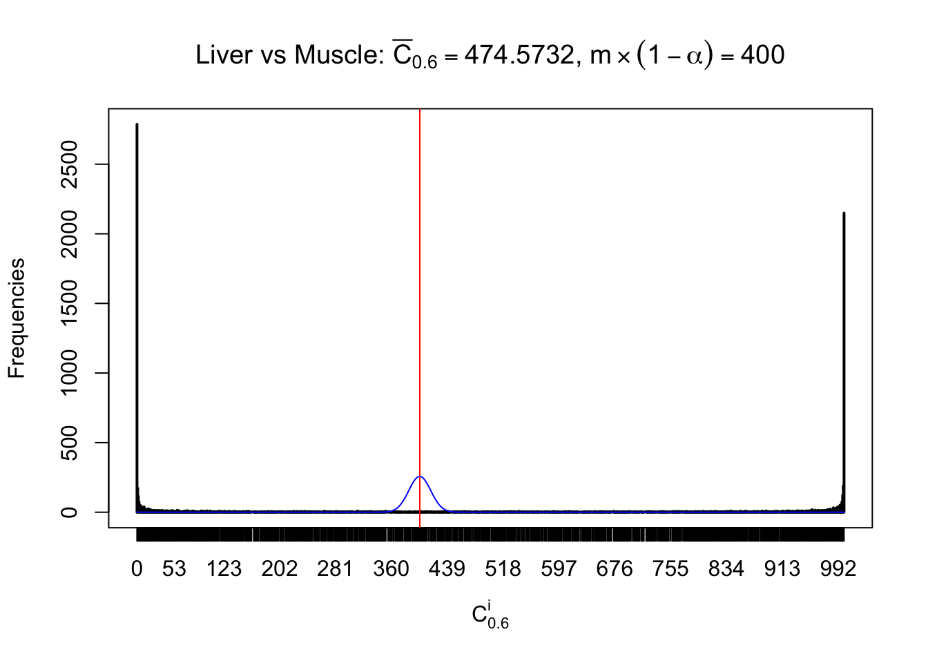
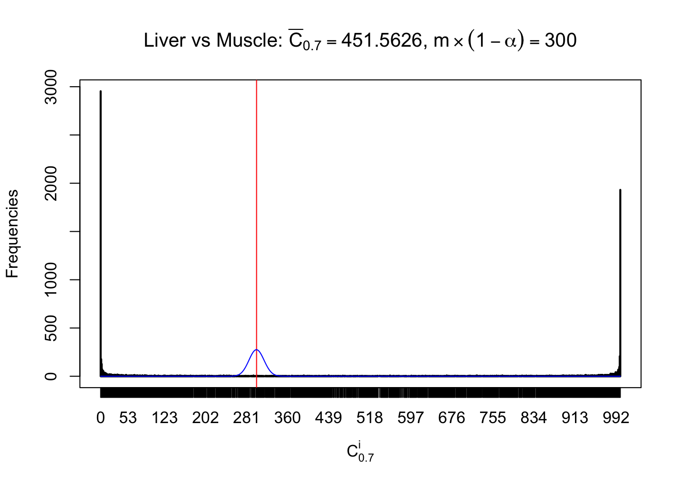
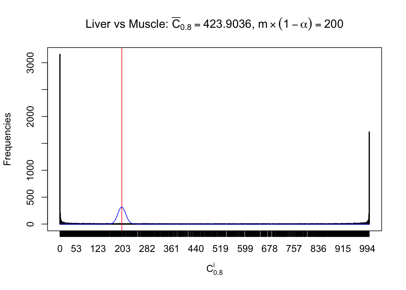
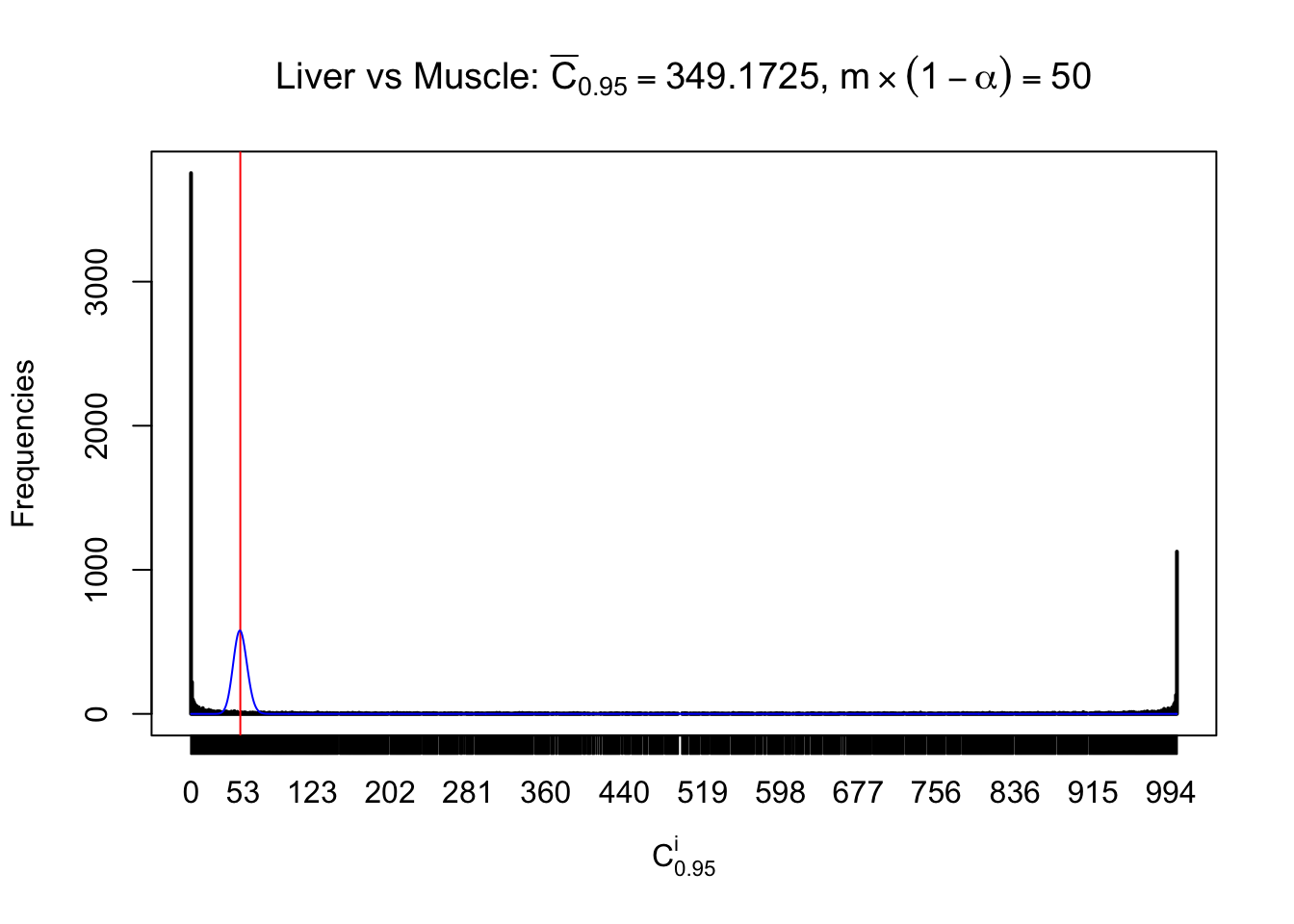
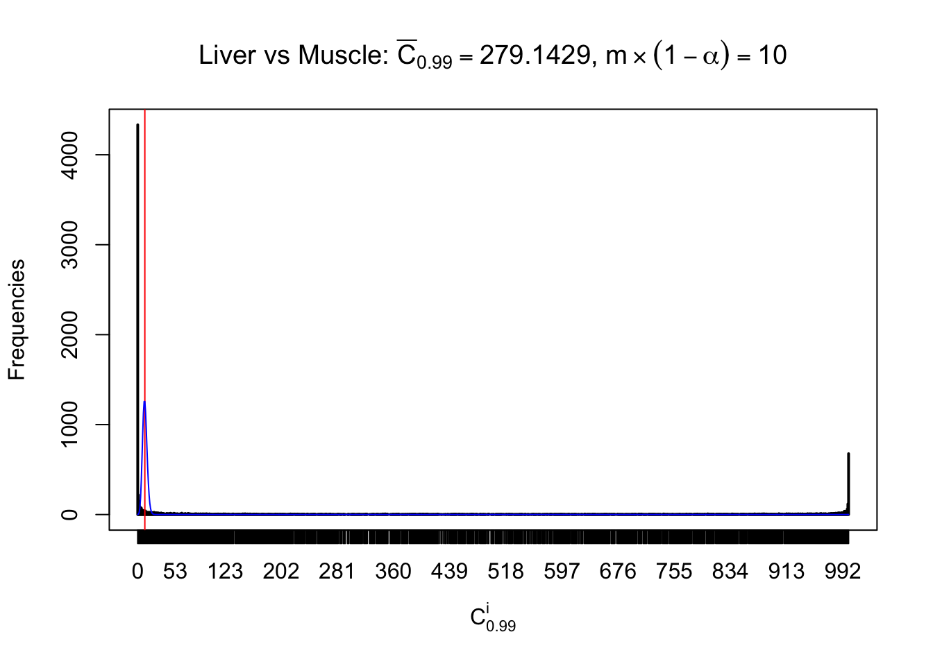
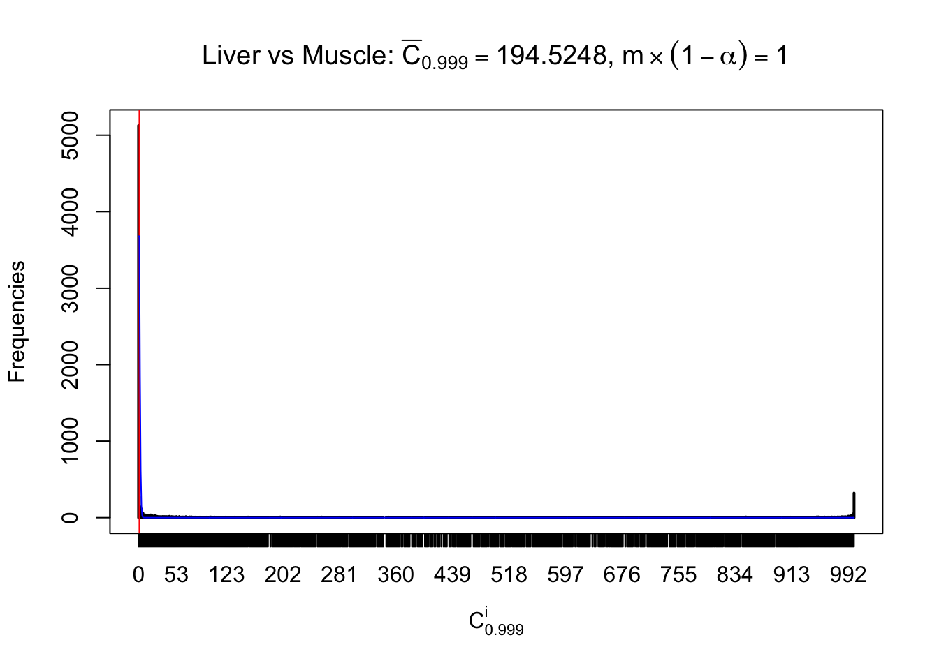
Liver vs Muscle
z.muscle = readRDS("../output/z_5liver_5muscle_777.rds")
n = ncol(z.muscle)
m = nrow(z.muscle)
Row-wise
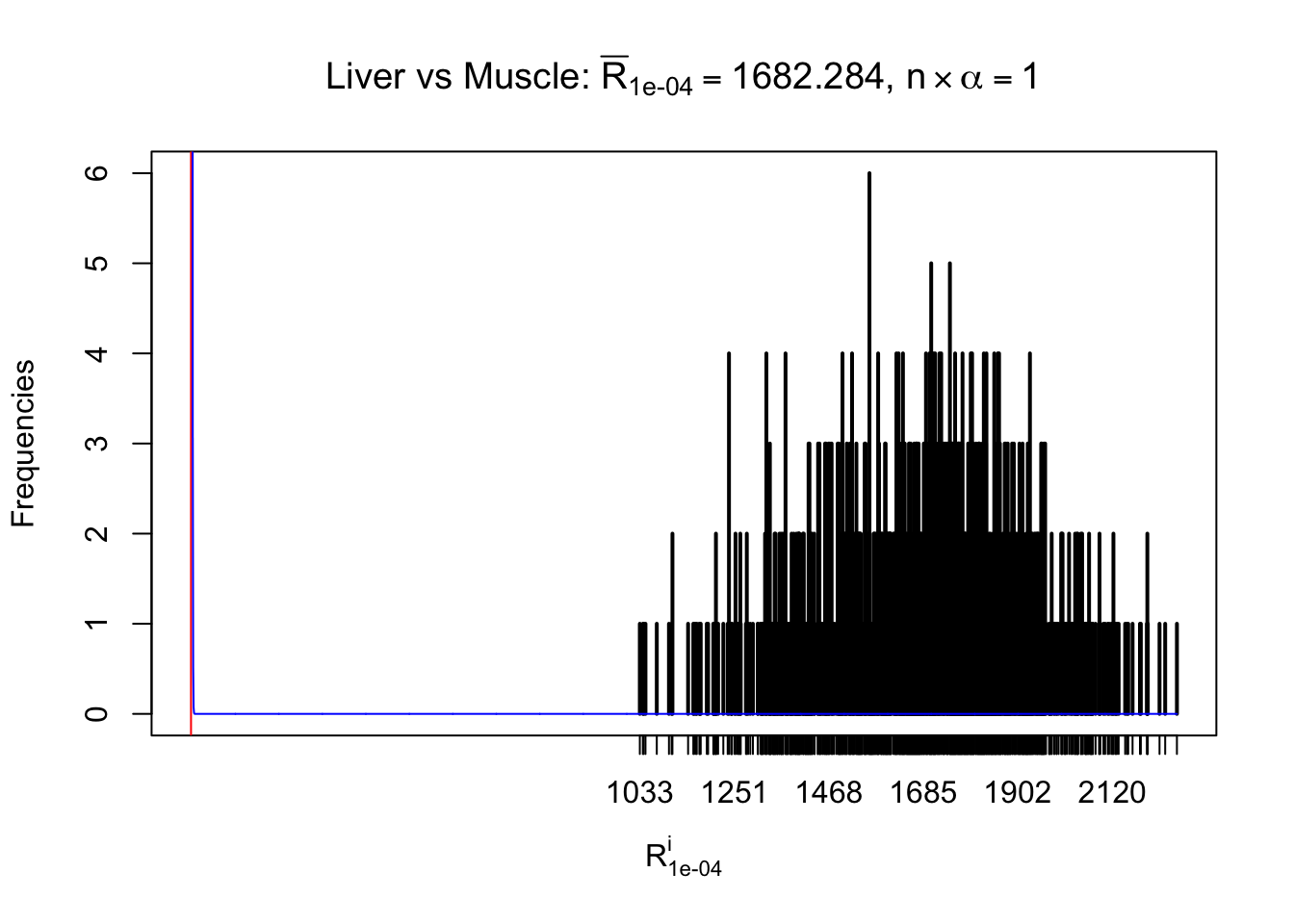
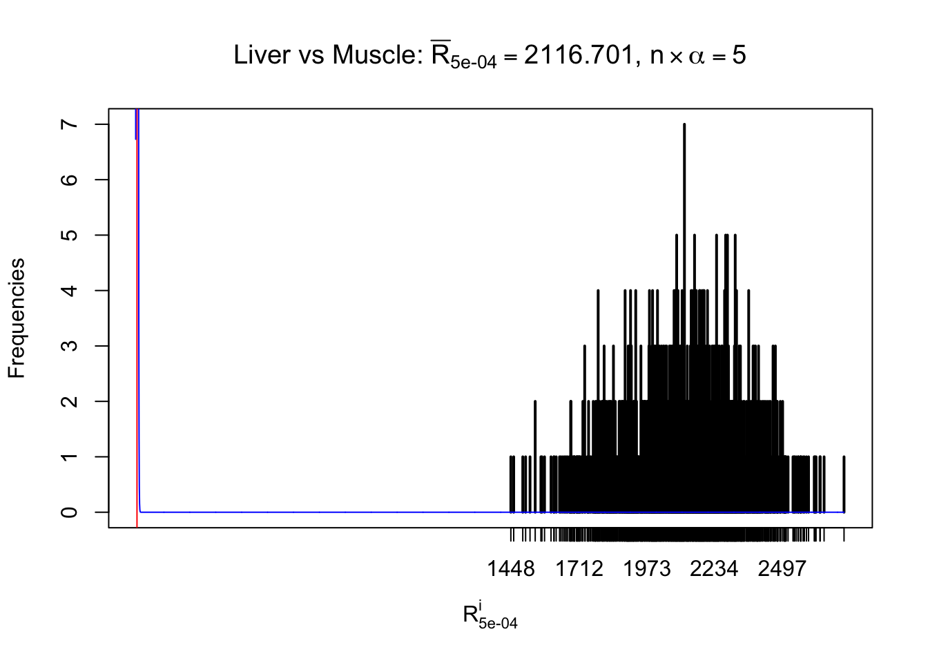
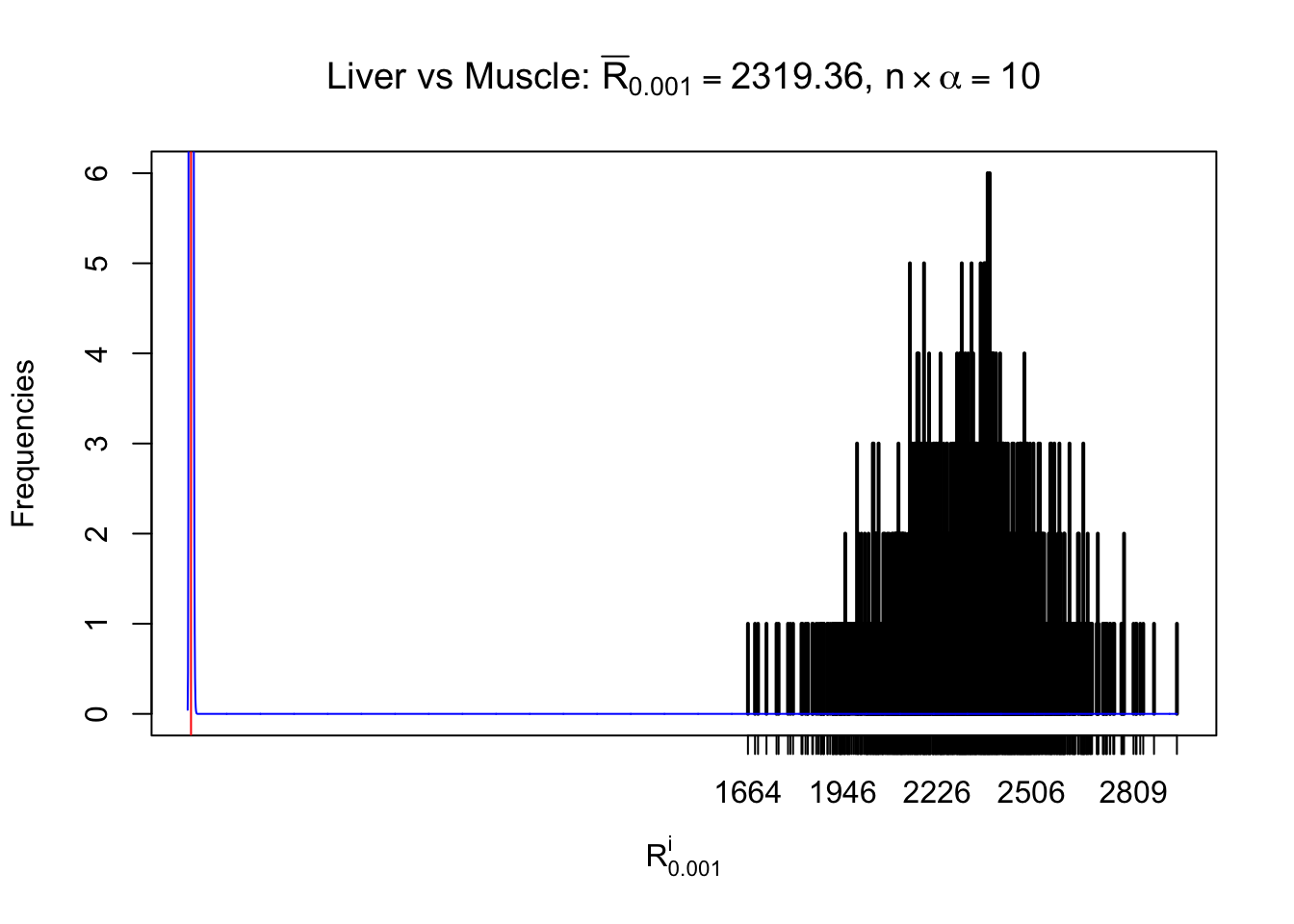
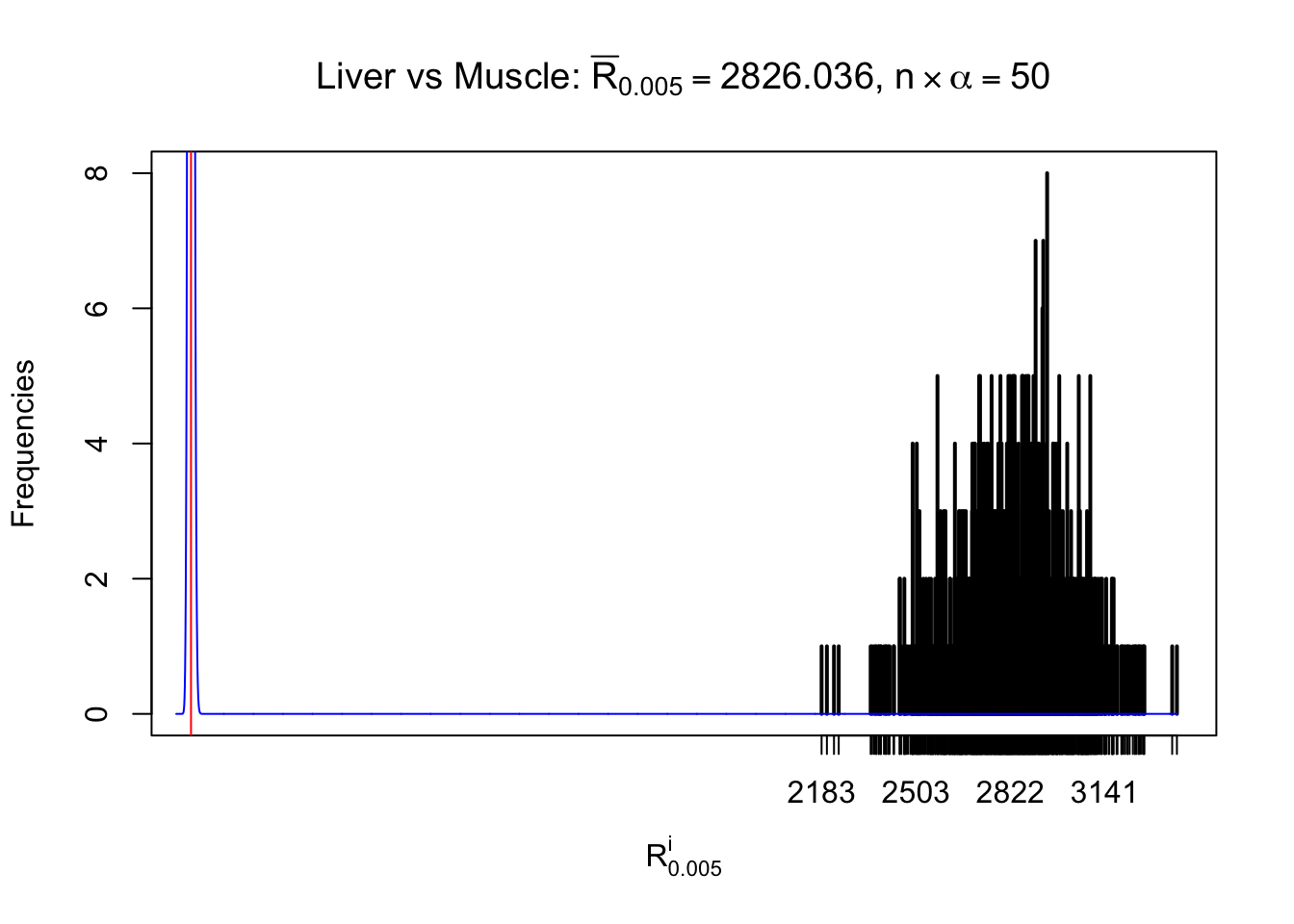
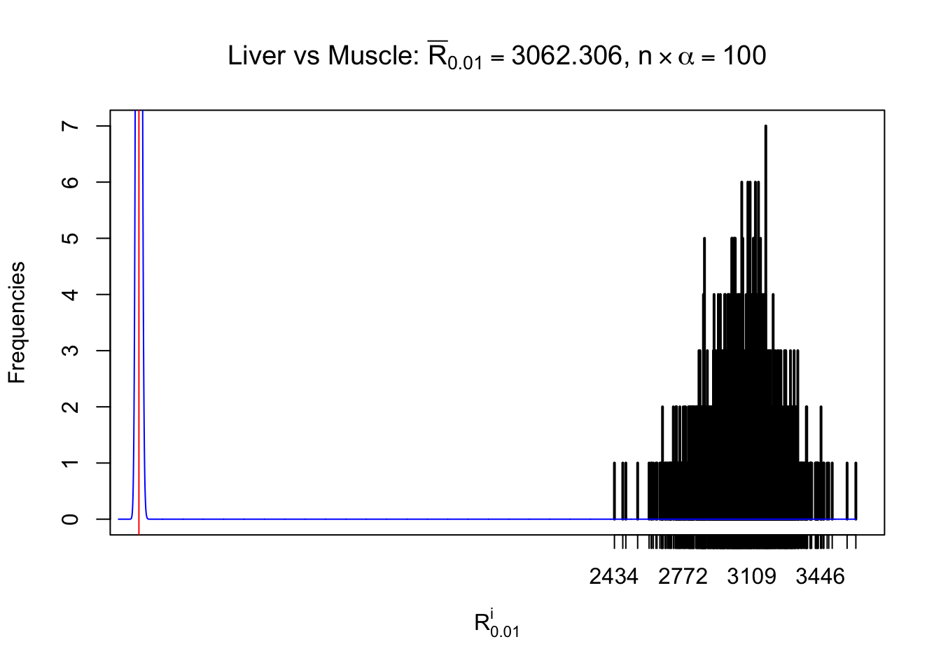
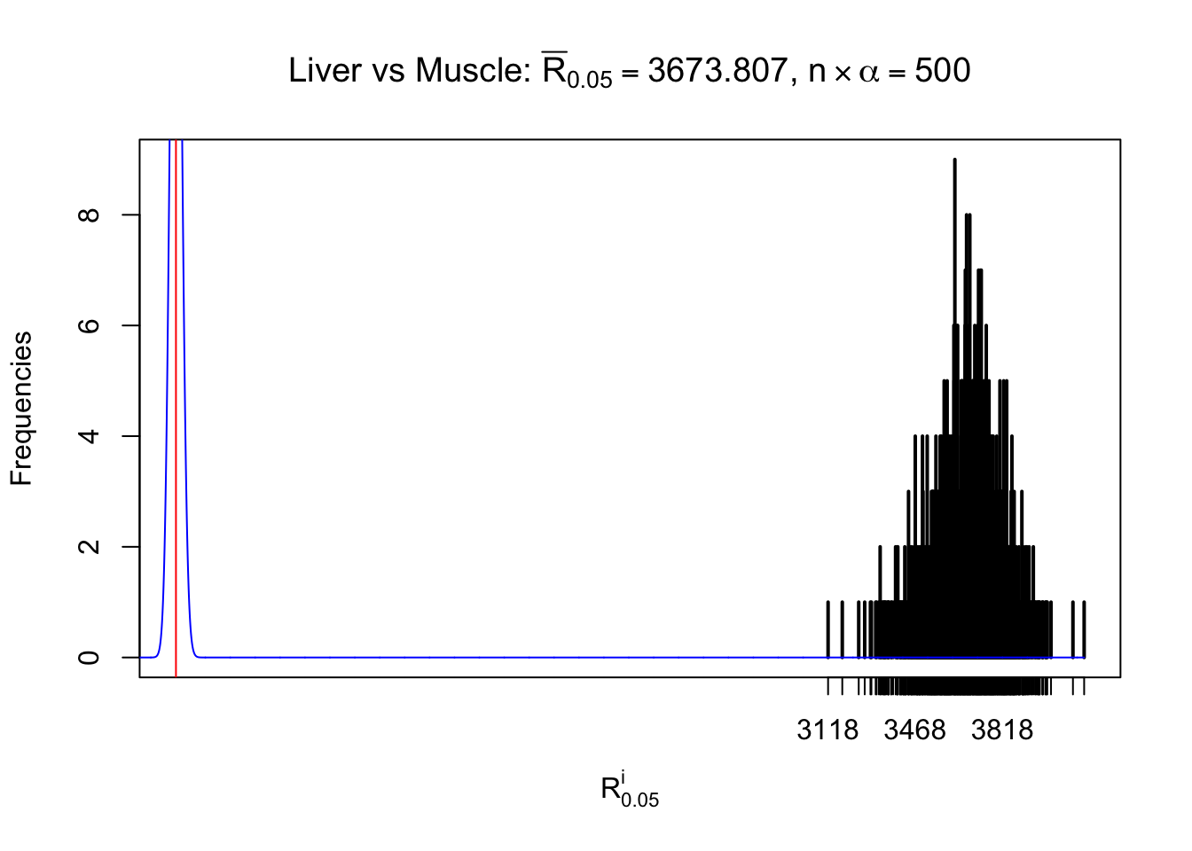
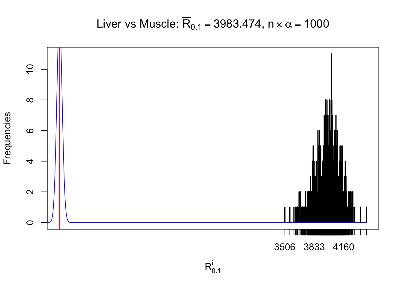

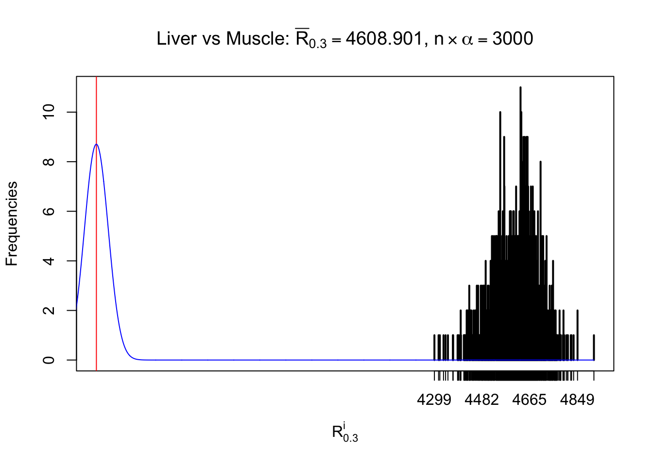
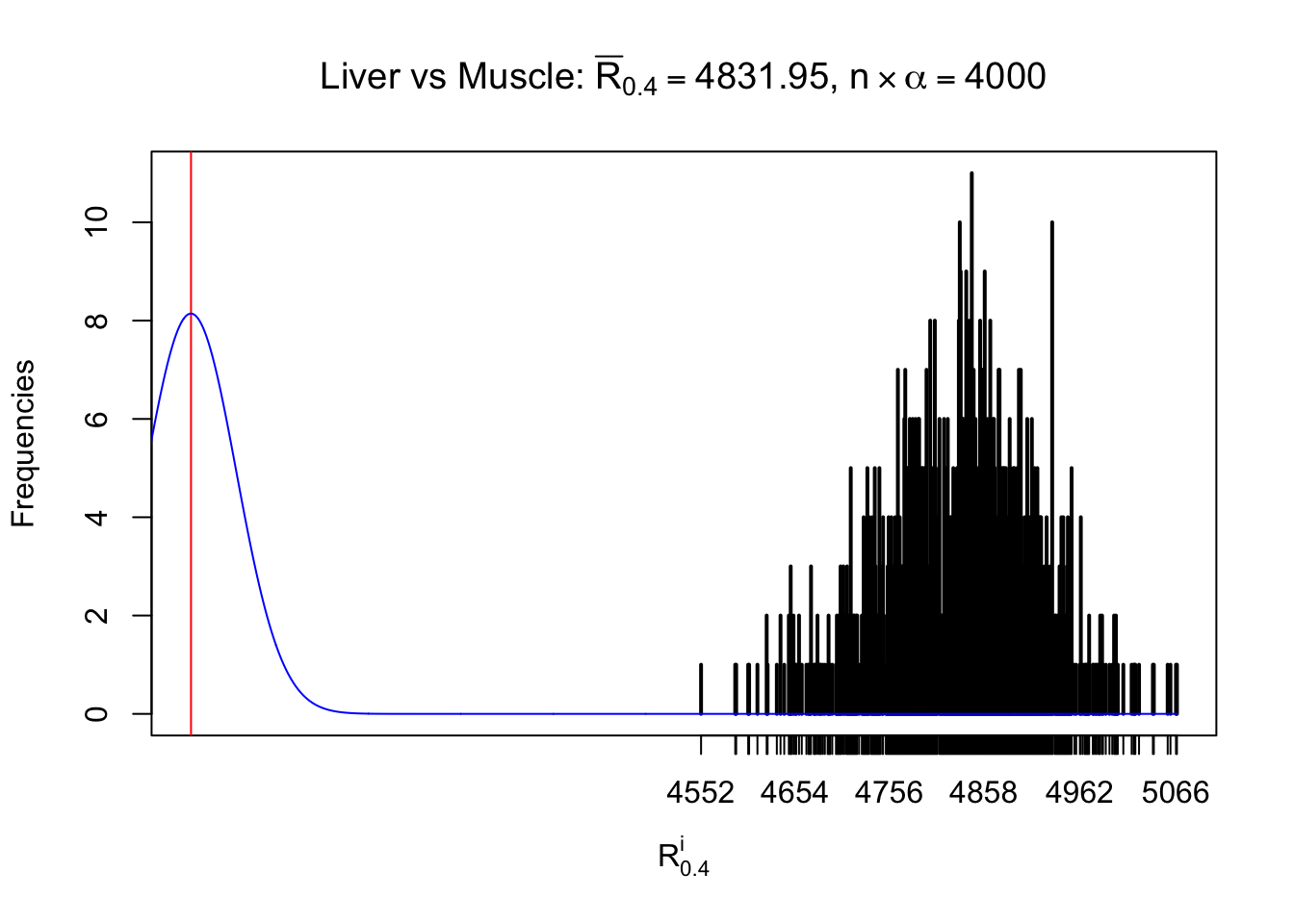
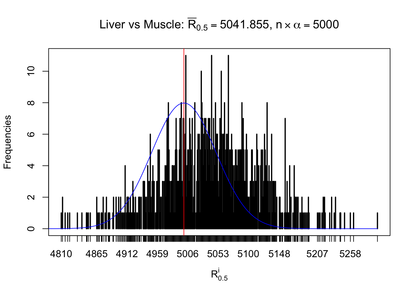
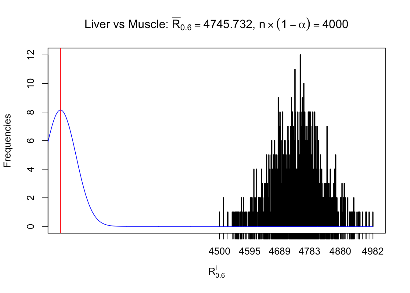
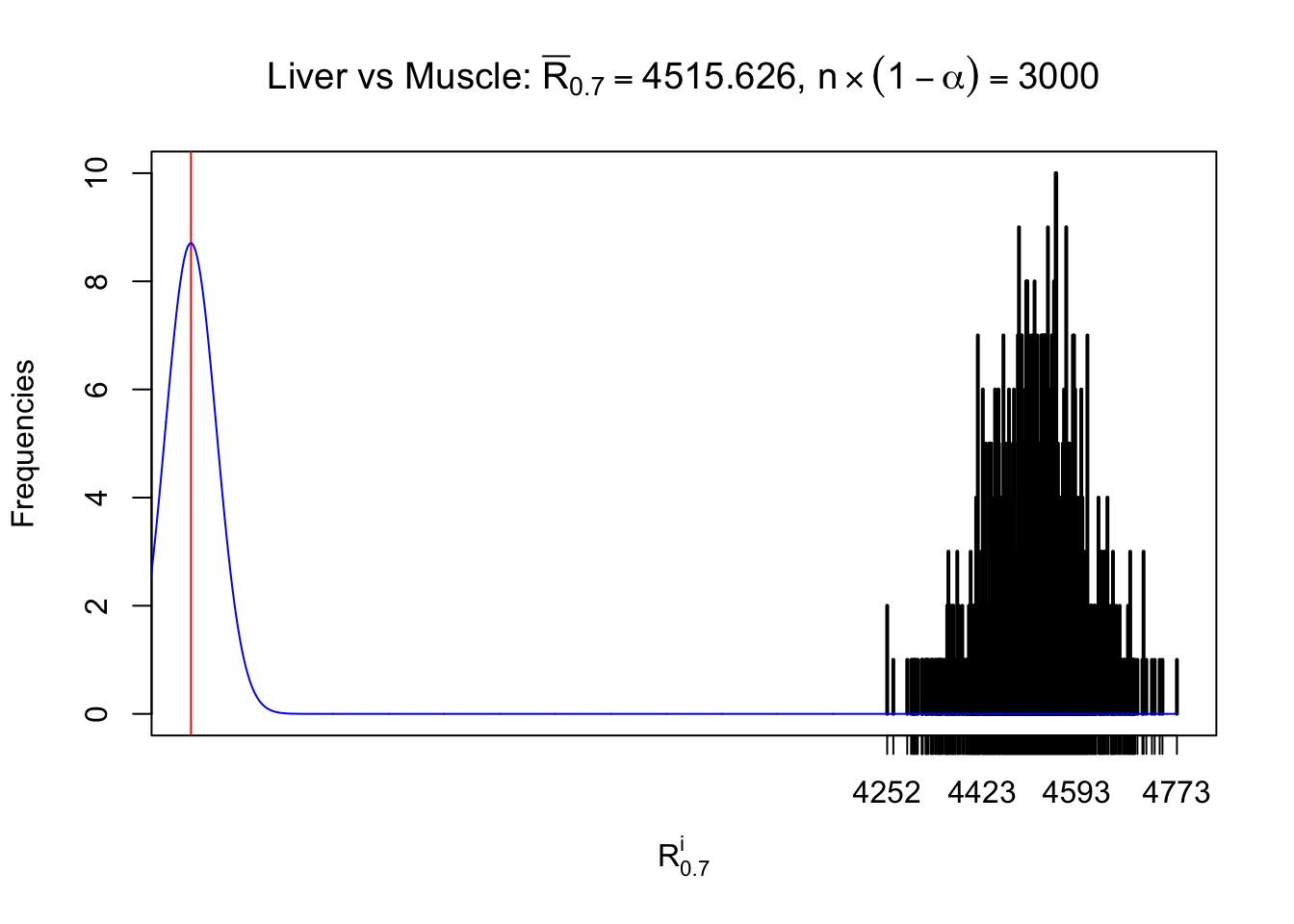

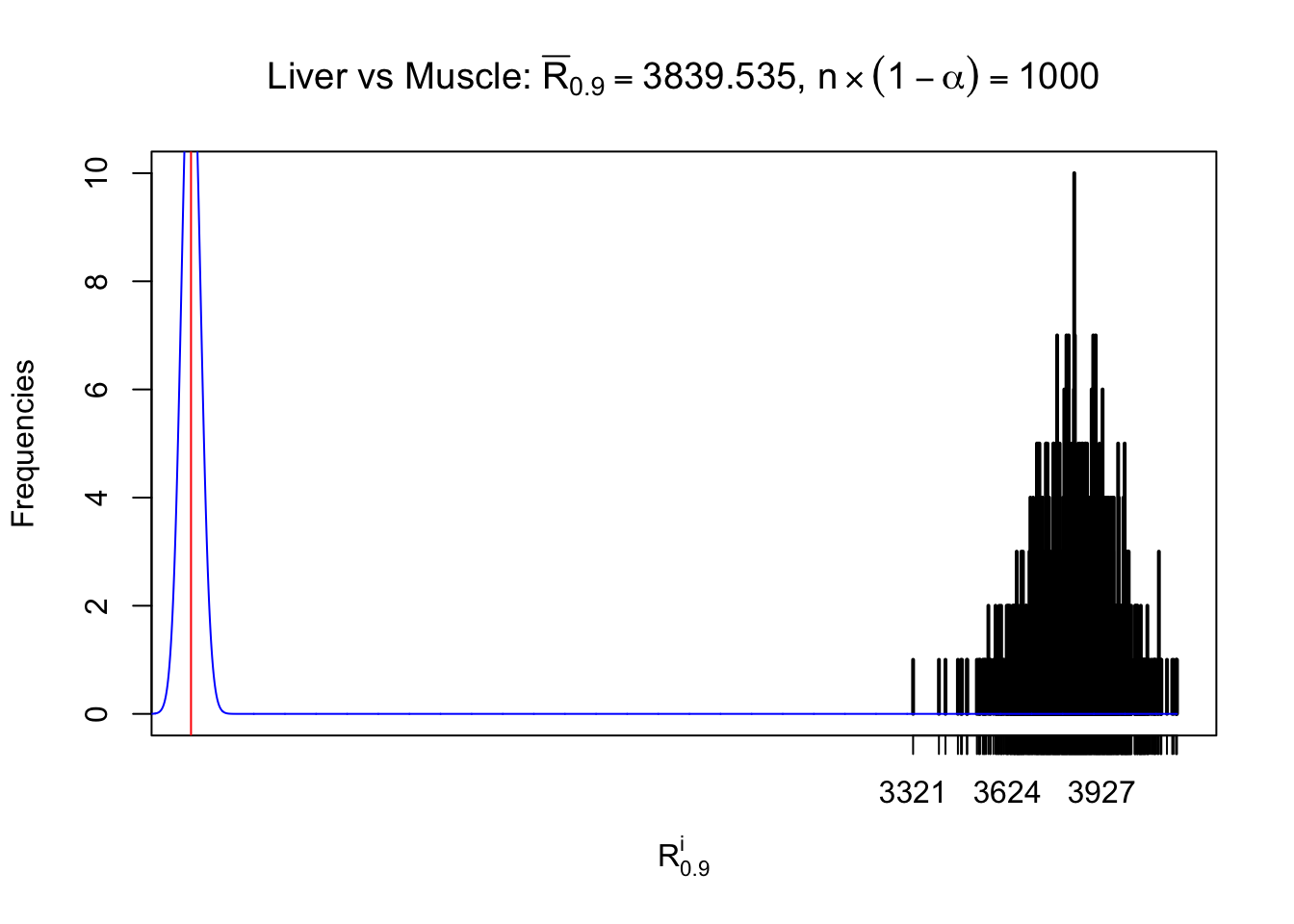
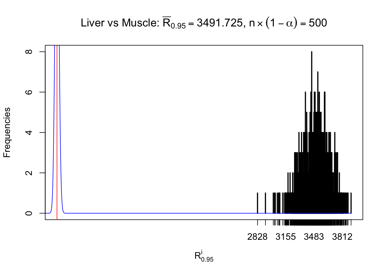
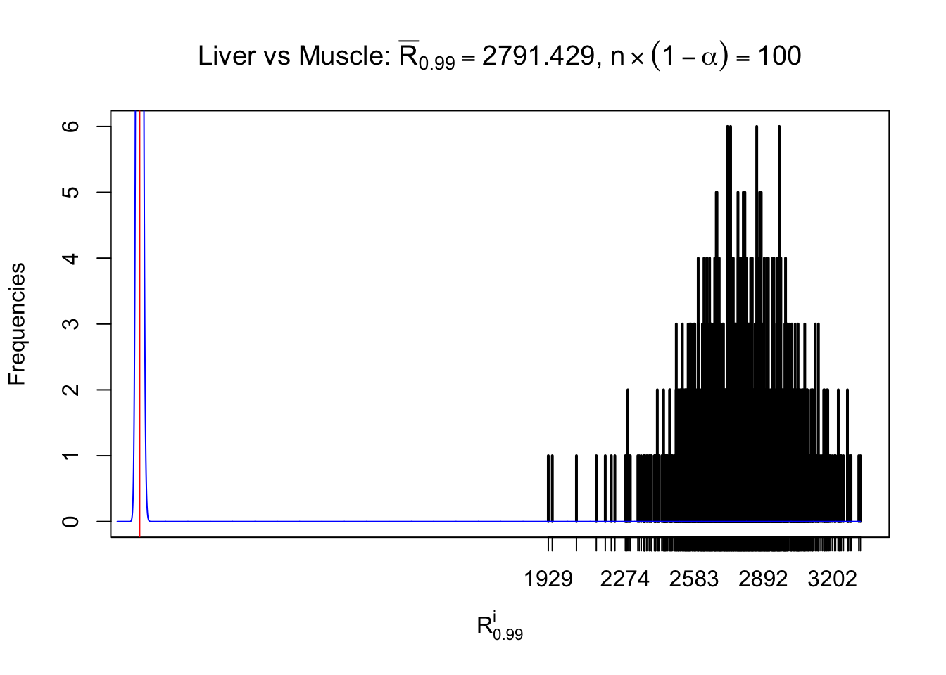
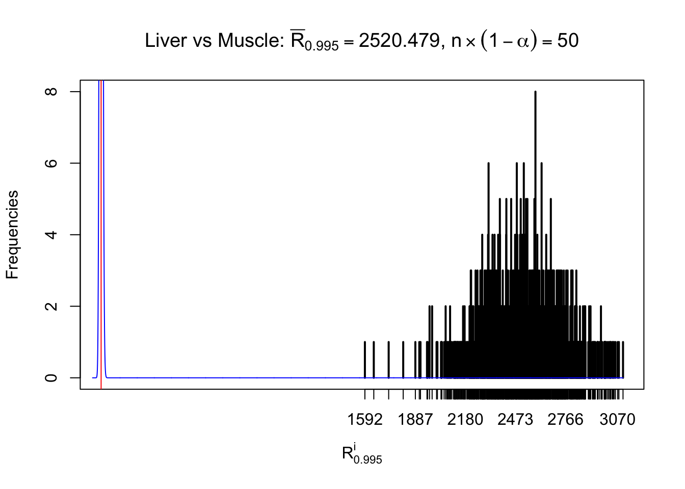
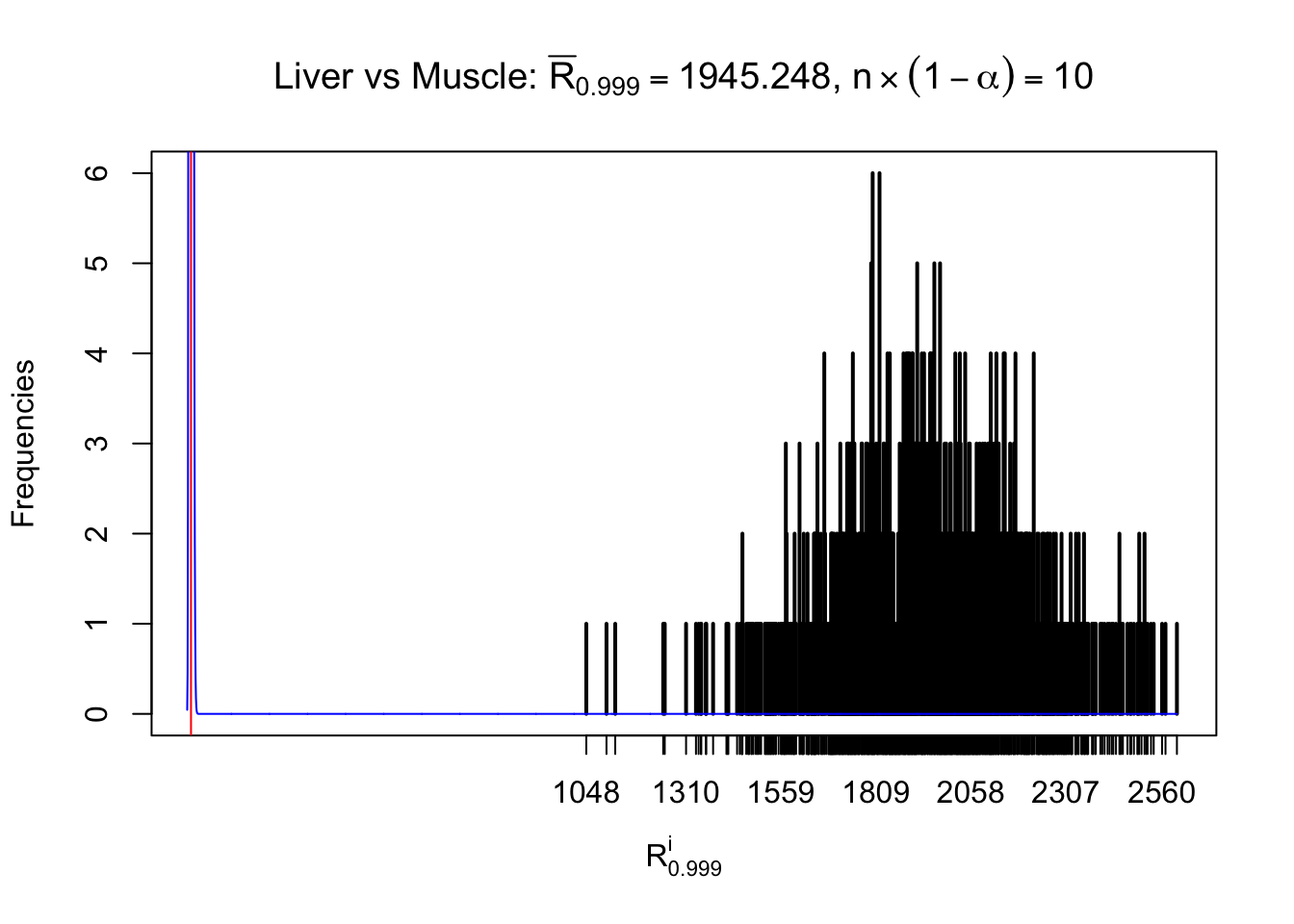
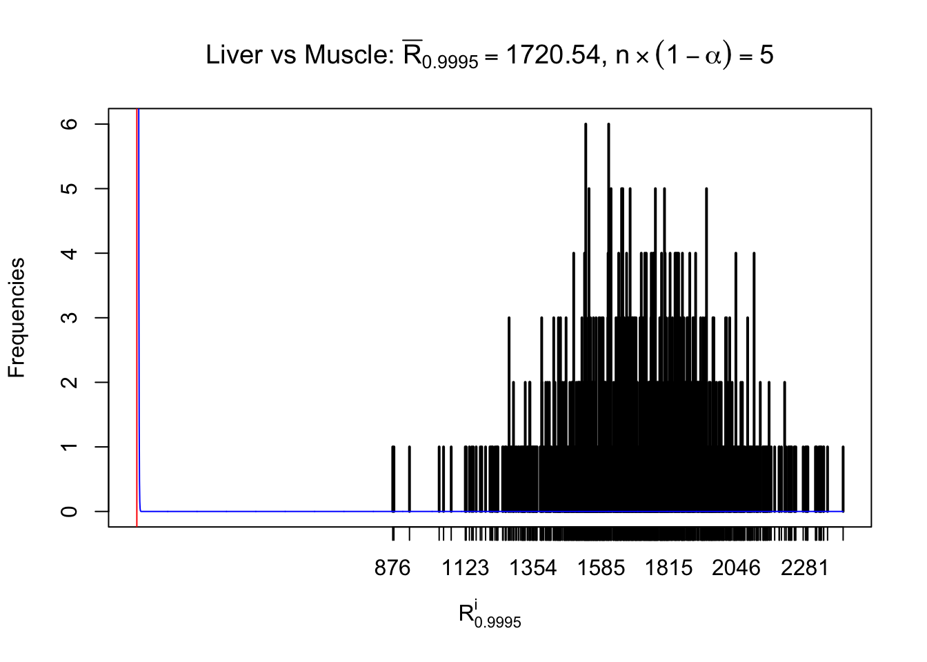
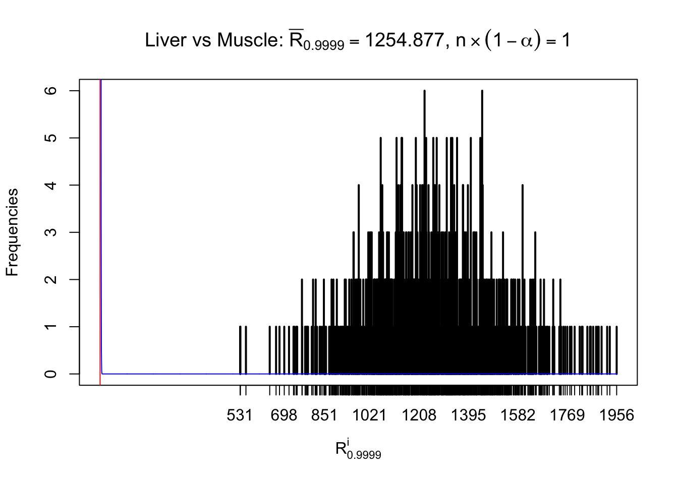
Column-wise


Conclusion
As expected, the empirical distribution and the indicated marginal distribution of the correlated non-null \(z\) scores are starkly different from those of the correlated null ones.
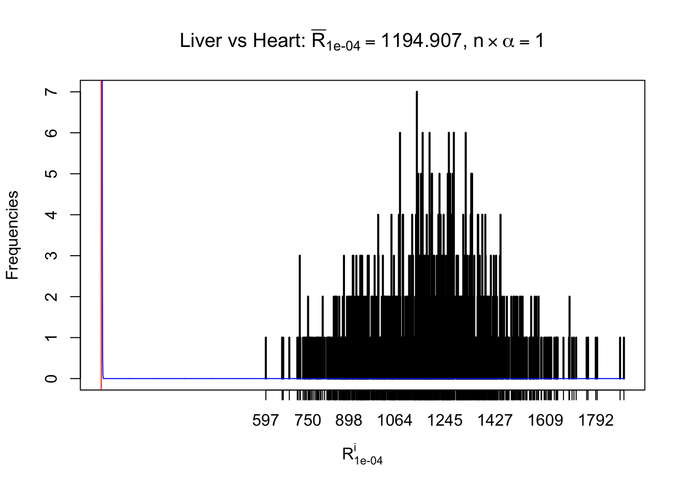
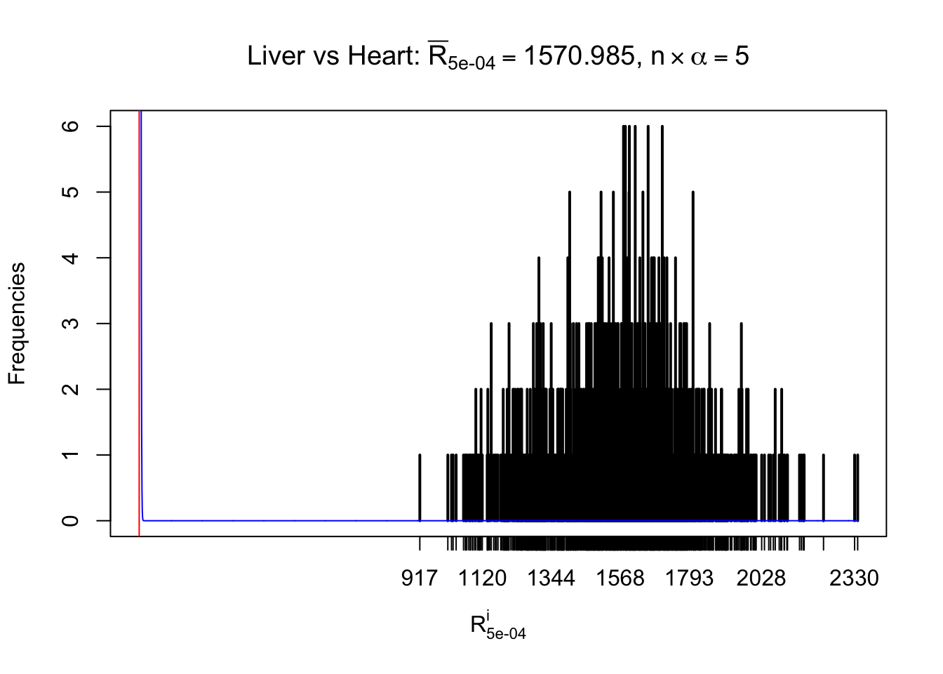
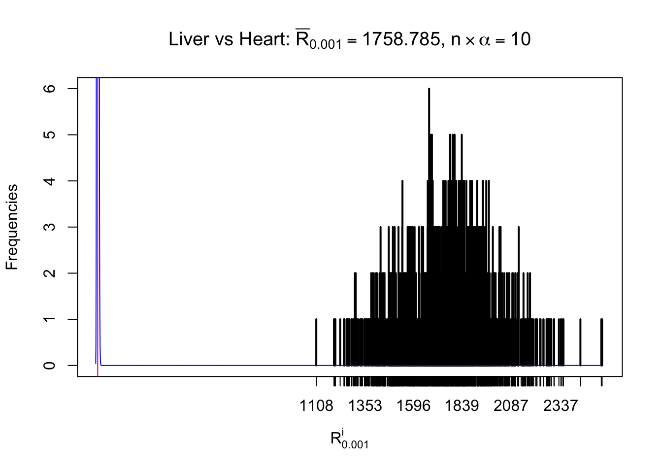
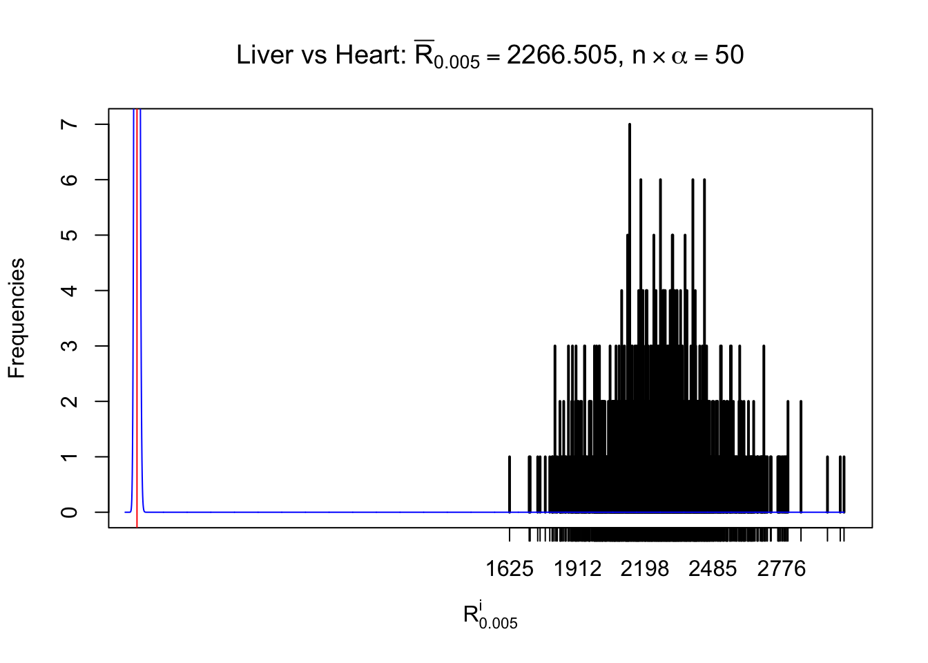
Particular interesting are the column-wise plots. The distribution of the number of tail observations is not only not close to normal, not close to what would be expected under correlated marginally \(N\left(0, 1\right)\), but also not even unimodal, not even peaked at \(m\alpha\) when \(\alpha \leq0.5\) or \(m\left(1-\alpha\right)\) when \(\alpha\geq0.5\). It suggests that there are indeed plenty of true signals, which make the marginal distribution of the \(z\) scores for a certain gene often not centered at \(0\).
Session information
sessionInfo()R version 3.4.3 (2017-11-30)
Platform: x86_64-apple-darwin15.6.0 (64-bit)
Running under: macOS High Sierra 10.13.2
Matrix products: default
BLAS: /Library/Frameworks/R.framework/Versions/3.4/Resources/lib/libRblas.0.dylib
LAPACK: /Library/Frameworks/R.framework/Versions/3.4/Resources/lib/libRlapack.dylib
locale:
[1] en_US.UTF-8/en_US.UTF-8/en_US.UTF-8/C/en_US.UTF-8/en_US.UTF-8
attached base packages:
[1] stats graphics grDevices utils datasets methods base
other attached packages:
[1] ashr_2.2-2 qvalue_2.10.0 edgeR_3.20.2 limma_3.34.4
loaded via a namespace (and not attached):
[1] Rcpp_0.12.14 compiler_3.4.3 git2r_0.20.0
[4] plyr_1.8.4 iterators_1.0.9 tools_3.4.3
[7] digest_0.6.13 evaluate_0.10.1 tibble_1.3.4
[10] gtable_0.2.0 lattice_0.20-35 rlang_0.1.4
[13] Matrix_1.2-12 foreach_1.4.4 yaml_2.1.16
[16] parallel_3.4.3 stringr_1.2.0 knitr_1.17
[19] locfit_1.5-9.1 rprojroot_1.3-1 grid_3.4.3
[22] rmarkdown_1.8 ggplot2_2.2.1 reshape2_1.4.3
[25] magrittr_1.5 backports_1.1.2 scales_0.5.0
[28] codetools_0.2-15 htmltools_0.3.6 splines_3.4.3
[31] MASS_7.3-47 colorspace_1.3-2 stringi_1.1.6
[34] lazyeval_0.2.1 munsell_0.4.3 doParallel_1.0.11
[37] pscl_1.5.2 truncnorm_1.0-7 SQUAREM_2017.10-1This R Markdown site was created with workflowr