Improvement on Implementation with Rmosek: Primal and Dual
Lei Sun
2017-05-07
Last updated: 2017-12-21
Code version: 6e42447
Introduction
We are experimenting different ways to improve the performance of Rmosek, using typical data sets of correlated \(z\) scores.
z <- read.table("../output/z_null_liver_777.txt")sel <- c(32, 327, 355, 483, 778)
ord <- c(4, 9, 9, 4, 4)source("../code/gdash.R")Algorithm and variations
Recall that our biconvex optimization problem is as follows.
\[ \begin{array}{rl} \min\limits_{\pi,w} & -\sum\limits_{j = 1}^n\log\left(\sum\limits_{k = 1}^K\sum\limits_{l=1}^L\pi_k w_l f_{jkl} + \sum\limits_{k = 1}^K\pi_kf_{jk0}\right) - \sum\limits_{k = 1}^K\left(\lambda_k^\pi - 1\right)\log\pi_k + \sum\limits_{l = 1}^L\lambda_l^w\phi\left(\left|w_l\right|\right) \\ \text{subject to} & \sum\limits_{k = 1}^K\pi_k = 1\\ & \sum\limits_{l=1}^L w_l \varphi^{(l)}\left(z\right) + \varphi\left(z\right) \geq 0, \forall z\in \mathbb{R}\\ & w_l \text{ decay reasonably fast,} \end{array} \] where \(- \sum\limits_{k = 1}^K\left(\lambda_k^\pi - 1\right)\log\pi_k\) and \(+ \sum\limits_{l = 1}^L\lambda_l^w\phi\left(\left|w_l\right|\right)\) are to regularize \(\pi_k\) and \(w_l\), respectively.
This problem can be solved iteratively. Starting with an initial value, each step two convex optimization problems are solved.
With a given \(\hat w\), \(\hat\pi\) is solved by
\[ \begin{array}{rl} \min\limits_{\pi} & -\sum\limits_{j = 1}^n\log\left(\sum\limits_{k = 1}^K\pi_k \left(\sum\limits_{l=1}^L \hat w_l f_{jkl} + f_{jk0}\right)\right) - \sum\limits_{k = 1}^K\left(\lambda_k^\pi - 1\right)\log\pi_k\\ \text{subject to} & \sum\limits_{k = 1}^K\pi_k = 1 \ ,\\ \end{array} \]
which is readily available with functions in cvxr.
Meanwhile, with a given \(\hat\pi\), the optimization problem to obtain \(\hat w\) becomes
\[ \begin{array}{rl} \min\limits_{w} & -\sum\limits_{j = 1}^n\log\left(\sum\limits_{l=1}^Lw_l\left(\sum\limits_{k = 1}^K\hat\pi_k f_{jkl}\right) + \sum\limits_{k = 1}^K\hat\pi_kf_{jk0}\right) + \sum\limits_{l = 1}^L\lambda_l^w \phi \left(\left|w_l\right|\right) \\ \text{subject to} & \sum\limits_{l=1}^L w_l \varphi^{(l)}\left(z\right) + \varphi\left(z\right) \geq 0, \forall z\in \mathbb{R}\\ & w_l \text{ decay reasonably fast.} \end{array} \] The two constraints are important to prevent numerical instability. Yet they are not readily manifested as convex. Ideally, the regularization \(\sum\limits_{l = 1}^L\lambda_l^w\phi\left(\left|w_l\right|\right)\) would be able to capture the essence of these two constaints, and at the same time maintain the convexity. Different ideas will be explored.
In this part, we’ll mainly work on the “basic form” of the \(w\) optimization problem; that is, the optimization problem without regularization \(\sum\limits_{l = 1}^L\lambda_l^w\phi\left(\left|w_l\right|\right)\).
In the following, we’ll take a look at the basic form in its primal and dual formulations, optimized by w.mosek() and w.mosek.primal functions. First, they are applied to the correlated null, and their performance can be compared with the previous implementation by cvxr. Then, they are applied to the simulated non-null data sets, and the results are compared with those obtained by ASH, as well as the truth.
Basic form: primal
In its most basic form, the \(w\) estimation problem is as follows.
\[ \begin{array}{rl} \min\limits_{w} & -\sum\limits_{j = 1}^n \log\left(\sum\limits_{l=1}^Lw_l a_{jl} + a_{j0}\right) \\ \text{subject to} & \sum\limits_{l=1}^Lw_l a_{jl} + a_{j0} \geq 0, \forall j \ .\\ \end{array} \] Let the matrix \(A = \left[a_{jl}\right]\), the vector \(a = \left[a_{j0}\right]\), and we have its equivalent form,
\[ \begin{array}{rl} \min\limits_{w, g} & -\sum\limits_{j = 1}^n \log\left(g_j\right) \\ \text{subject to} & Aw + a = g \\ & g \geq 0\ . \end{array} \]
This problem can be coded by Rmosek as a “separable convex optimization” (SCOPT) problem.
Correlated null
Fitted w: -0.03653526 0.1999284 0.01047094 -0.02012681
Time Cost in Seconds: 7.945 2.884 13.152 
Fitted w: 0.03394291 0.7345604 -0.1532514 0.1883912 -0.05504895 0.02297176 -0.006908406 0.001216017 -0.0003147927
Time Cost in Seconds: 6.902 1.98 6.669 
Fitted w: 0.02262546 0.9213963 0.02180428 0.1760983 -0.01379674 0.003968132 -0.004904973 -0.0006085249 -0.0002990675
Time Cost in Seconds: 5.375 1.932 6.116 
Fitted w: 0.04540484 -0.1275978 0.009150985 0.01004515
Time Cost in Seconds: 19.294 2.066 14.959 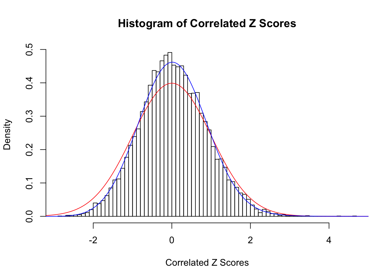
Fitted w: 0.005943196 0.3980709 -0.009222458 0.02630697
Time Cost in Seconds: 6.636 1.954 6.815 
Signal \(+\) correlated error
Converged: FALSE
Number of Iteration: 101
Time Cost in Seconds: 2181.997 255.051 1644.499 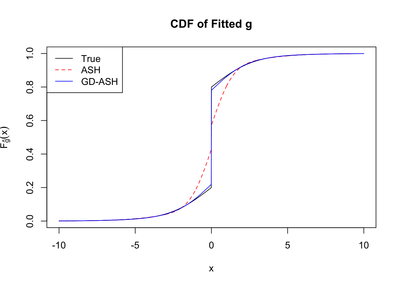
Converged: FALSE
Number of Iteration: 101
Time Cost in Seconds: 2634.559 296.365 1970.452 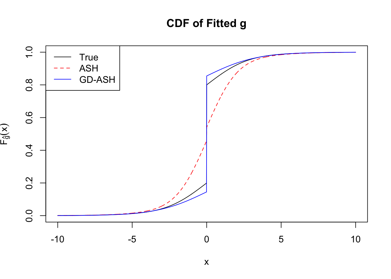
Converged: TRUE
Number of Iteration: 45
Time Cost in Seconds: 553.188 127.588 540.733 
Converged: TRUE
Number of Iteration: 49
Time Cost in Seconds: 781.062 126.839 622.938 
Converged: FALSE
Number of Iteration: 101
Time Cost in Seconds: 2161.426 247.628 1565.216 
Basic form: dual
The primal \(w\) optimization problem has \(n + L\) variables and \(n\) constraints. When \(n\) is large, such as \(n = 10K\) in our simulations, the time cost is usually substantial. As the authors of REBayes pointed out, it’s better to work on the dual form, which is
\[ \begin{array}{rl} \min\limits_{v} & -\sum\limits_{j = 1}^n \log\left(v_j\right) + a^Tv \\ \text{subject to} & A^Tv = 0 \\ & v \geq 0\ . \end{array} \] The dual form has \(n\) variables and more importantly, only \(L\) constraints. As \(L \ll n\), the dual form is far more computationally efficient.
Rmosek provides optimal solutions to both primal and dual variables, so \(\hat w\) is readily available when working on \(v\) optimization. But we need to be careful on which dual variables to use, such as $sol$itr$suc, $sol$itr$slc, or others.
Correlated null
Fitted w: -0.03642797 0.1971637 0.01074601 -0.02181494
Time Cost in Seconds: 0.485 0.049 0.388 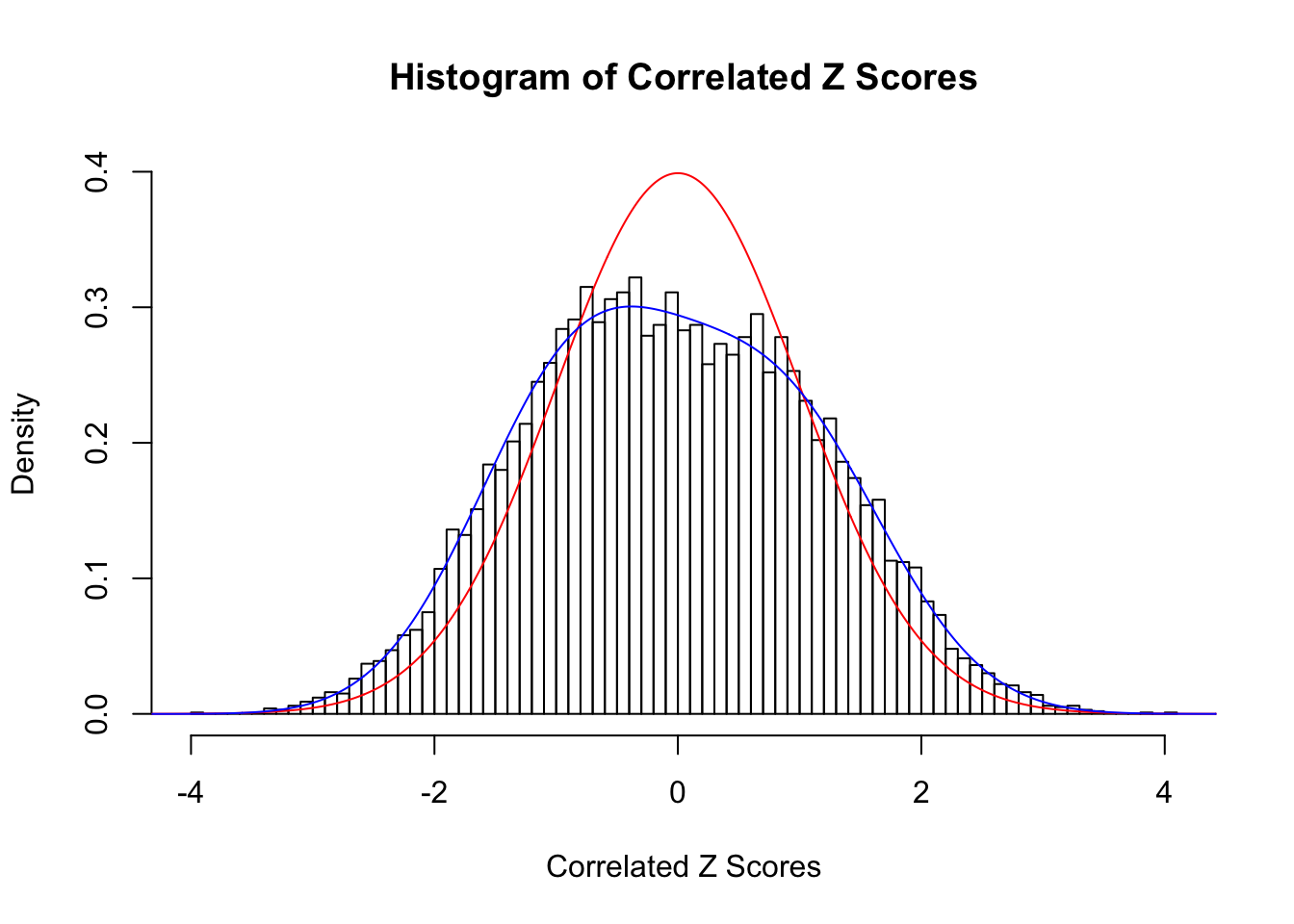
Fitted w: 0.03361434 0.7339189 -0.1544144 0.1875235 -0.0560049 0.02267003 -0.007151714 0.001187682 -0.0003321398
Time Cost in Seconds: 0.524 0.009 0.372 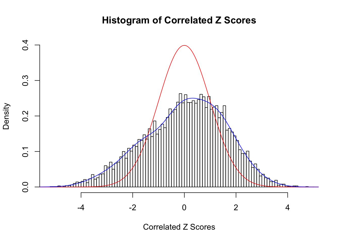
Fitted w: 0.02273596 0.9206369 0.02224234 0.1750273 -0.01339113 0.003607418 -0.004794795 -0.0006395078 -0.0002908422
Time Cost in Seconds: 0.529 0.008 0.375 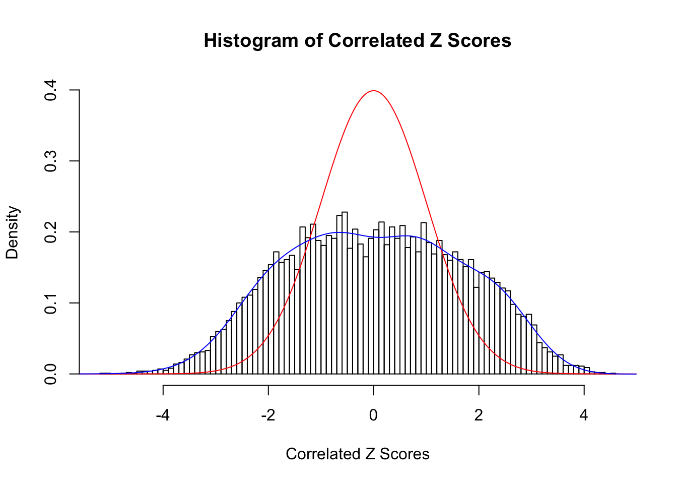
Fitted w: 0.04544396 -0.1272823 0.008811108 0.009915311
Time Cost in Seconds: 0.448 0.006 0.322 
Fitted w: 0.006084177 0.3976595 -0.009103231 0.02610567
Time Cost in Seconds: 0.489 0.005 0.313 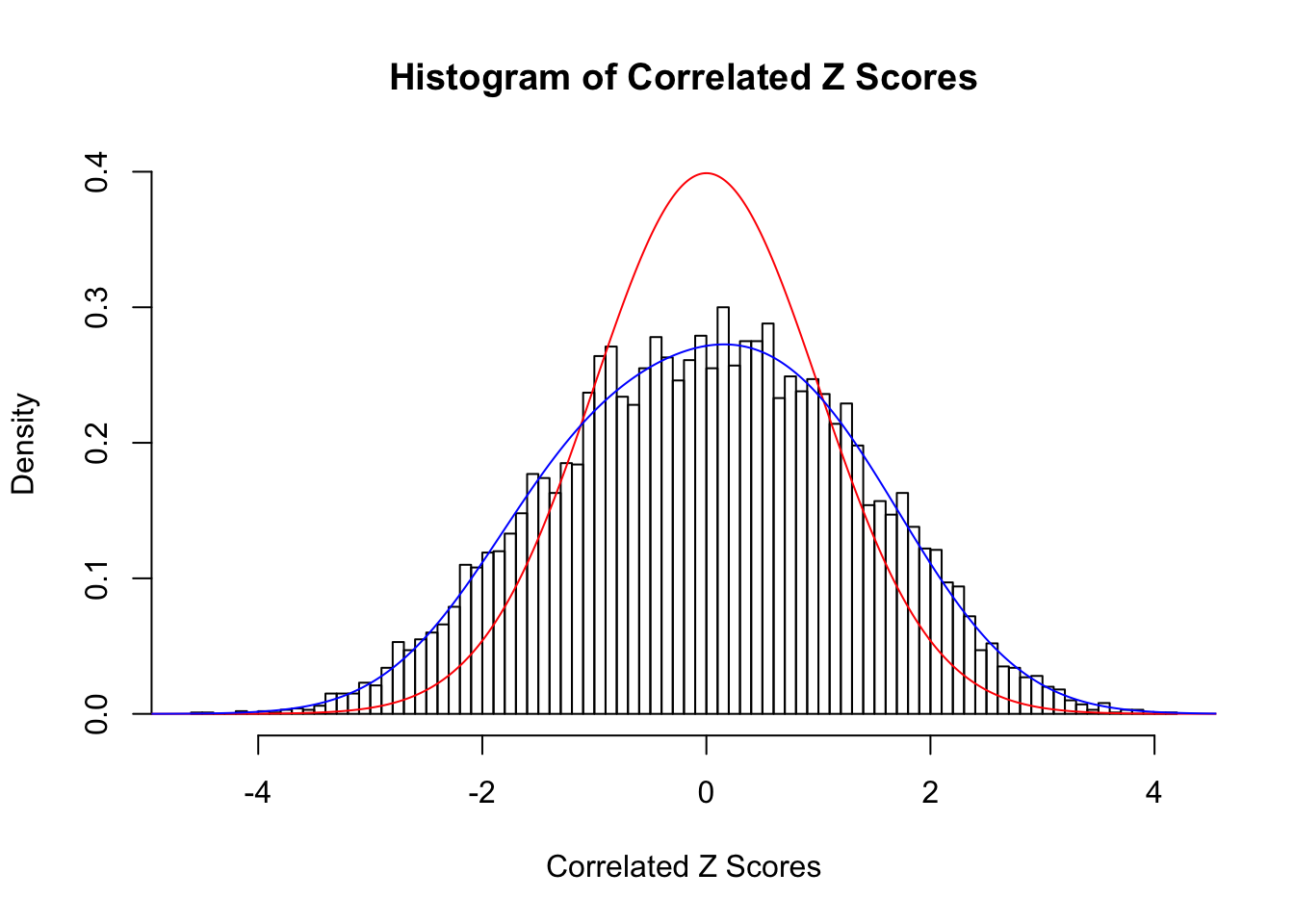
Signal \(+\) correlated error
Converged: TRUE
Number of Iteration: 21
Time Cost in Seconds: 46.978 2.71 29.017 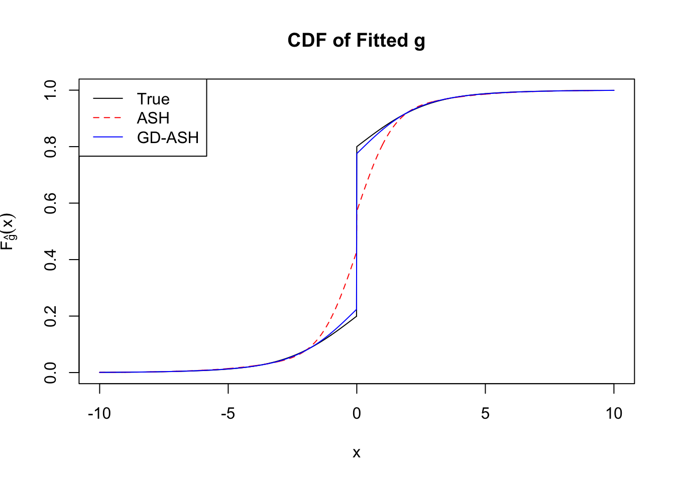
Converged: TRUE
Number of Iteration: 21
Time Cost in Seconds: 45.406 5.343 52.01 
Converged: TRUE
Number of Iteration: 16
Time Cost in Seconds: 34.293 3.519 26.79 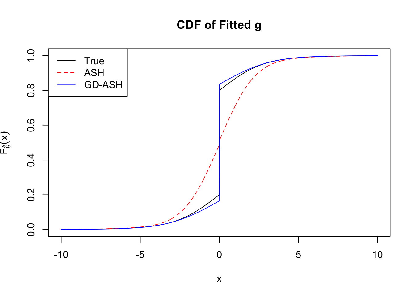
Converged: TRUE
Number of Iteration: 31
Time Cost in Seconds: 64.198 3.902 39.897 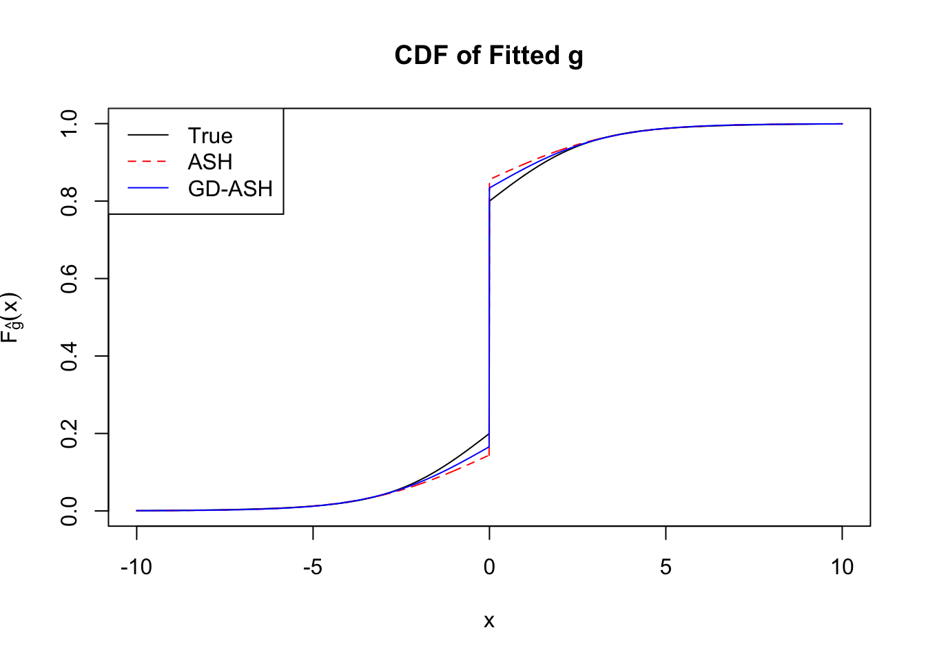
Converged: TRUE
Number of Iteration: 12
Time Cost in Seconds: 27.247 1.446 15.392 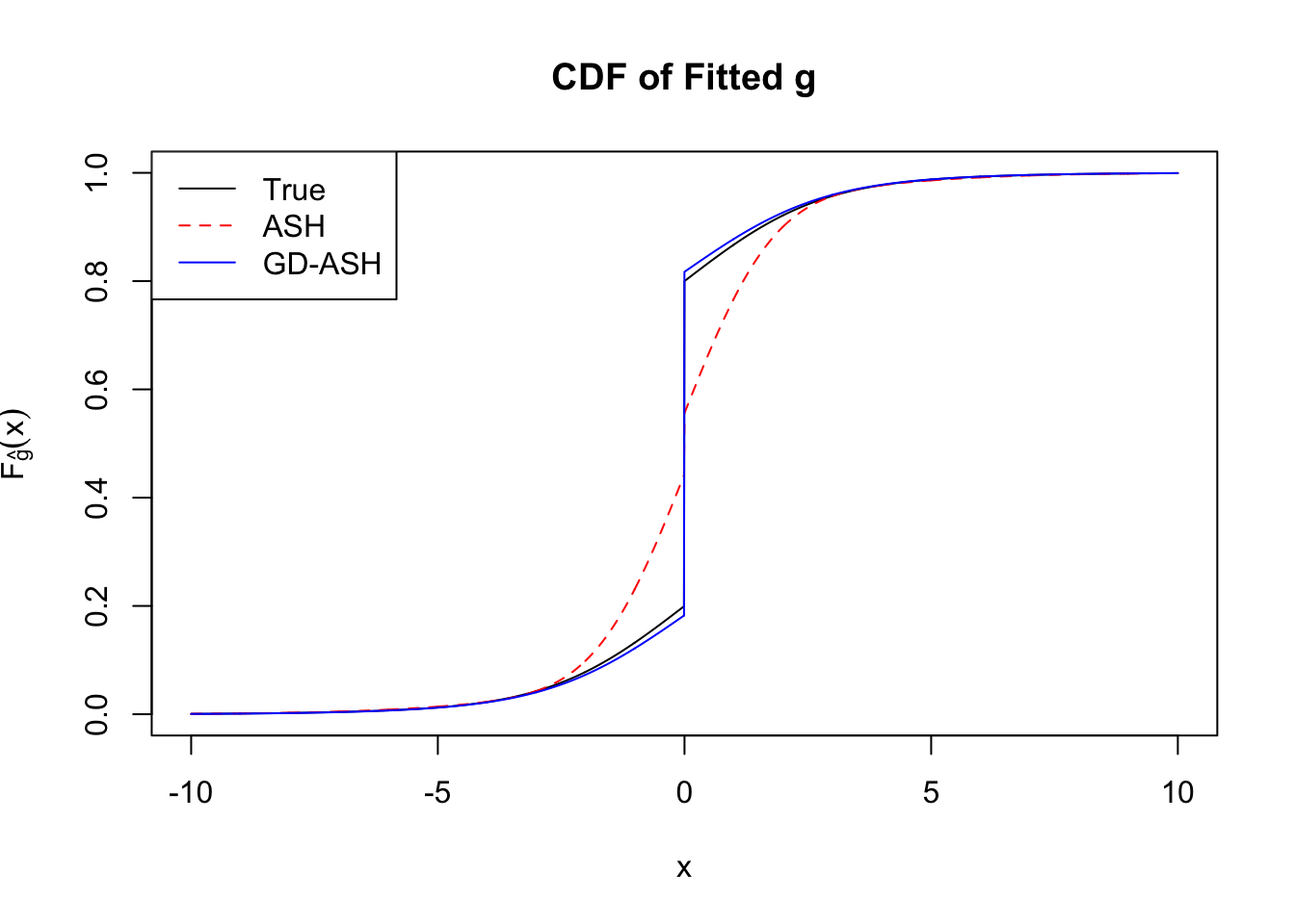
Conclusion
Implementation by Rmosek can fully reproduce the results obtained by cvxr. Moreover, the dual form gives the same results as the primal dorm does, with only a fraction of time.
It seems hopeful that we’ll find a key to successfully tackle correlation in simultaneous inference, which has eluded Prof. Brad Efron for more than a decade.
Session information
sessionInfo()R version 3.4.3 (2017-11-30)
Platform: x86_64-apple-darwin15.6.0 (64-bit)
Running under: macOS High Sierra 10.13.2
Matrix products: default
BLAS: /Library/Frameworks/R.framework/Versions/3.4/Resources/lib/libRblas.0.dylib
LAPACK: /Library/Frameworks/R.framework/Versions/3.4/Resources/lib/libRlapack.dylib
locale:
[1] en_US.UTF-8/en_US.UTF-8/en_US.UTF-8/C/en_US.UTF-8/en_US.UTF-8
attached base packages:
[1] stats graphics grDevices utils datasets methods base
other attached packages:
[1] Rmosek_8.0.69 PolynomF_1.0-1 CVXR_0.94-4 REBayes_1.2
[5] Matrix_1.2-12 SQUAREM_2017.10-1 EQL_1.0-0 ttutils_1.0-1
loaded via a namespace (and not attached):
[1] Rcpp_0.12.14 knitr_1.17 magrittr_1.5
[4] bit_1.1-12 lattice_0.20-35 R6_2.2.2
[7] stringr_1.2.0 tools_3.4.3 grid_3.4.3
[10] R.oo_1.21.0 git2r_0.20.0 scs_1.1-1
[13] htmltools_0.3.6 bit64_0.9-7 yaml_2.1.16
[16] rprojroot_1.3-1 digest_0.6.13 gmp_0.5-13.1
[19] ECOSolveR_0.3-2 R.utils_2.6.0 evaluate_0.10.1
[22] rmarkdown_1.8 stringi_1.1.6 compiler_3.4.3
[25] Rmpfr_0.6-1 backports_1.1.2 R.methodsS3_1.7.1This R Markdown site was created with workflowr