plot_diagnostic in ashr

Introduction

This file documents some simulations done for a May 12, 2017, NHS presentation on the diagnostic plots for ASH implemented by ashr::plot_diagnostic().

library(ashr)
library(qvalue)

The concept of a Q-Q plot

set.seed(777)
x = rnorm(100)
qqnorm(x)
qqline(x)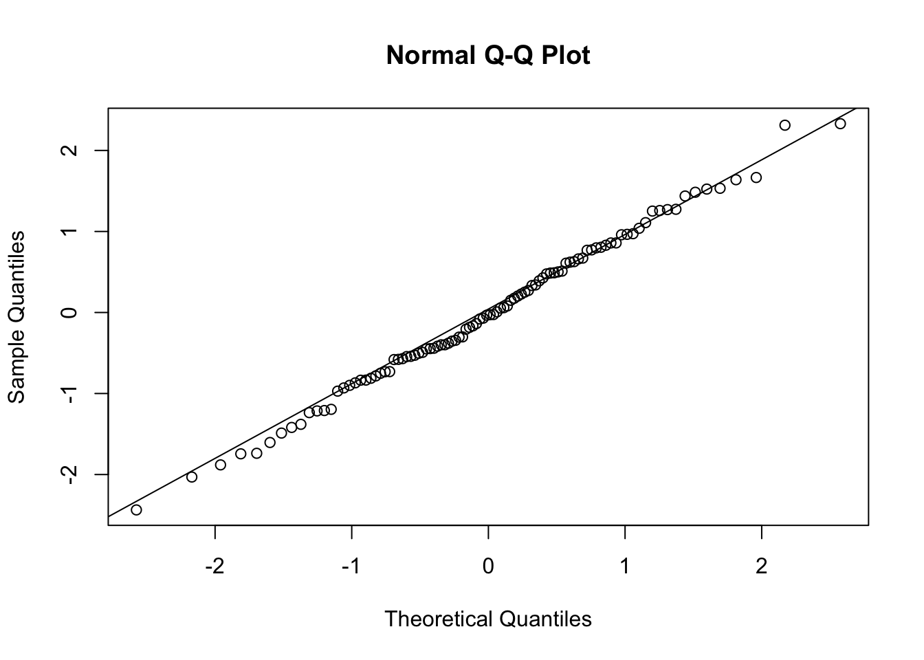

y = runif(100)
qqnorm(y)
qqline(y)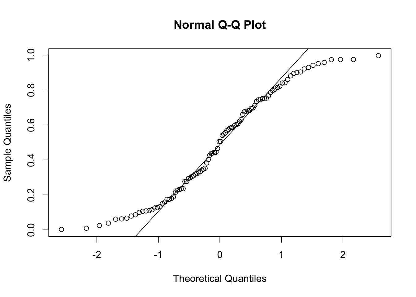

Diagnostic plots for ASH applied to different data sets

beta = runif(10000)
betahat = beta + rnorm(10000)
fit = ash(betahat, 1, mixcompdist = "normal", method = "fdr")
plot_diagnostic(fit)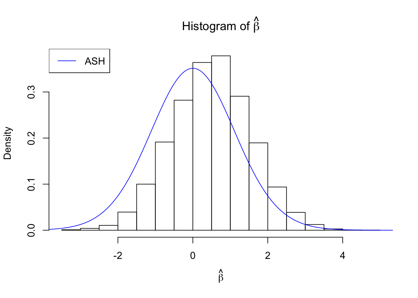

Press [enter] to see next plot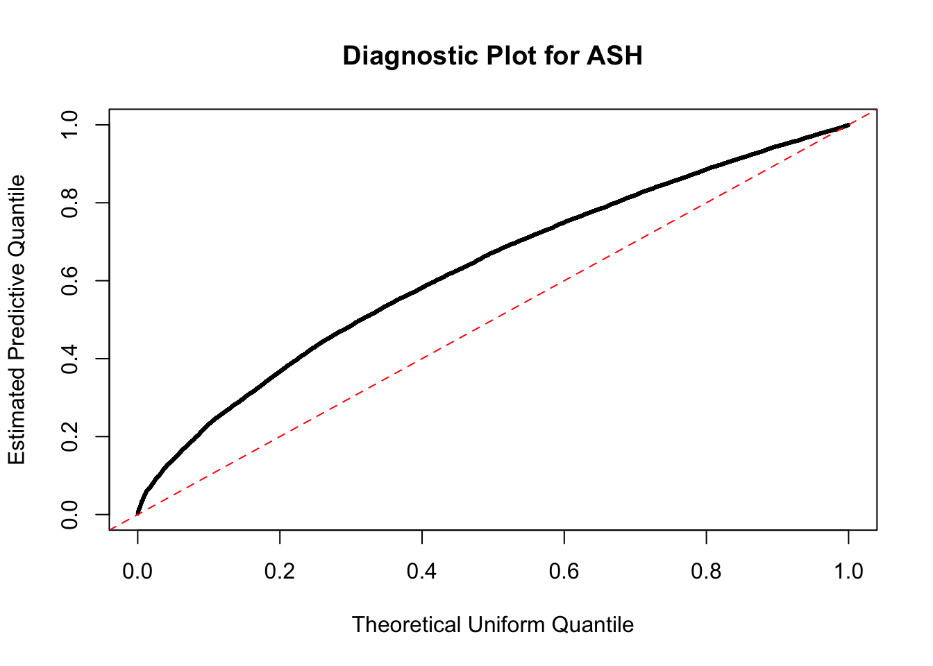

Press [enter] to see next plot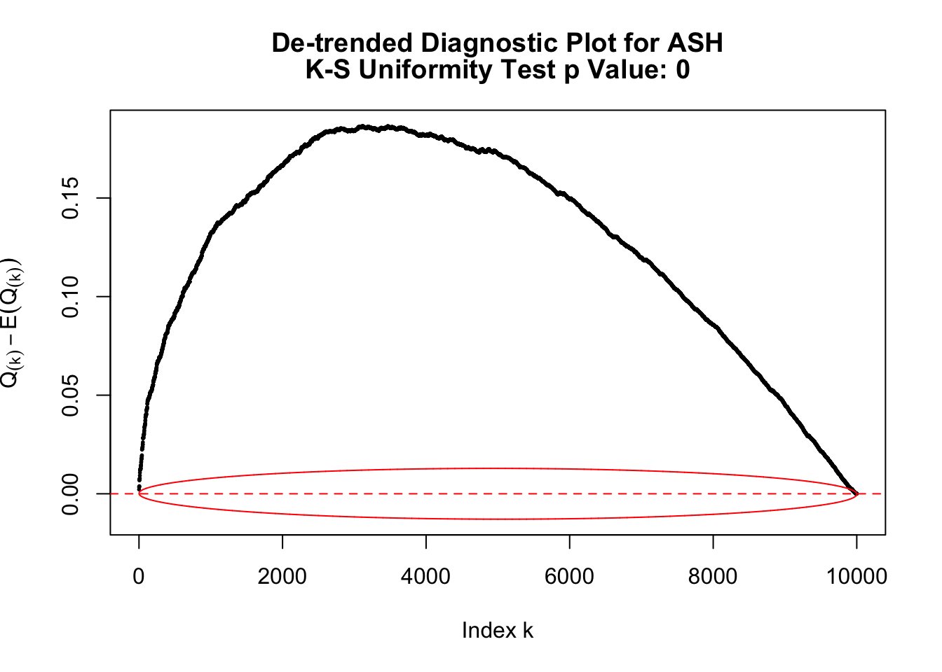

Press [enter] to see next plot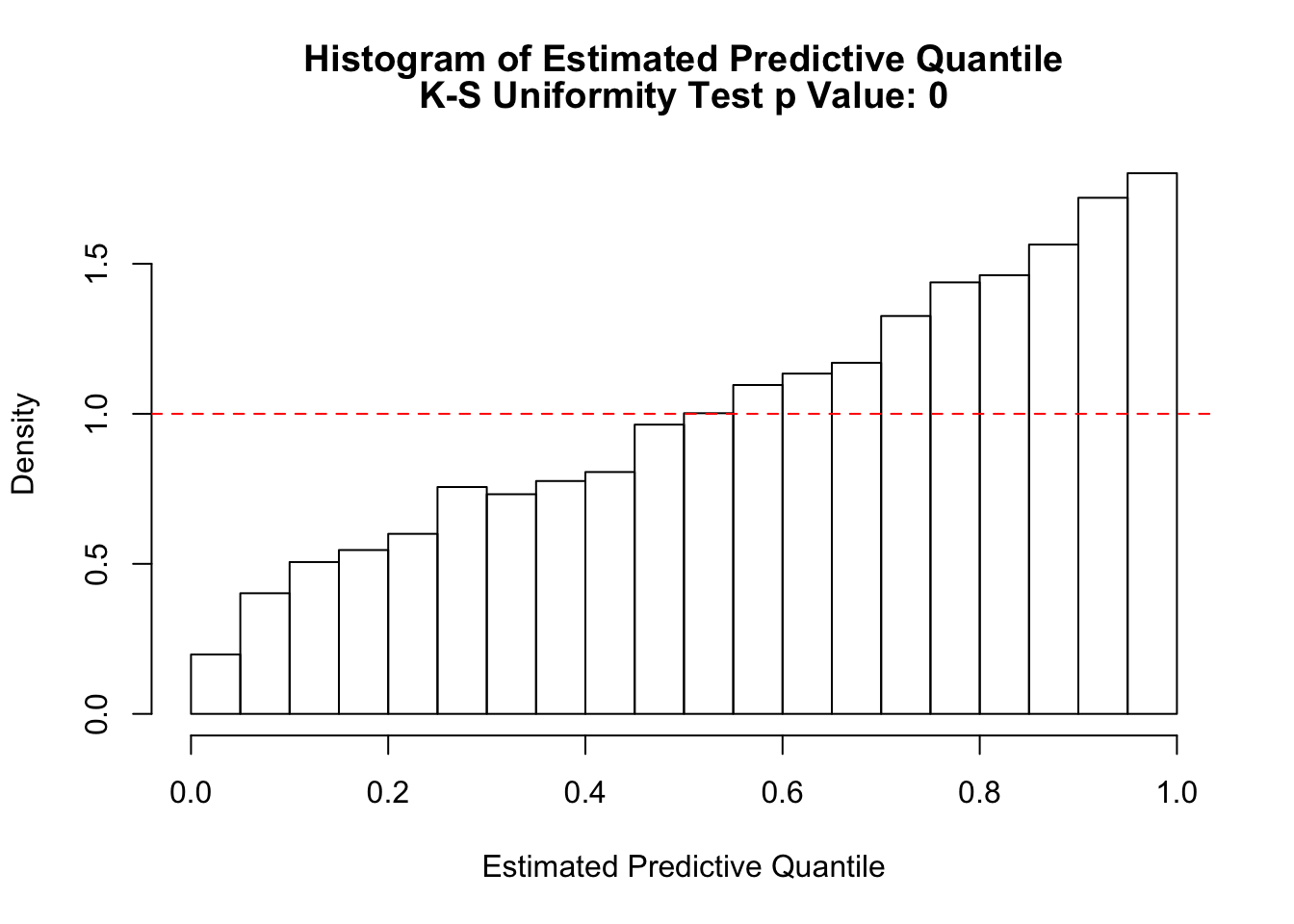

par(mfrow = c(2, 2))
fit = ash(rnorm(10000), 1, mixcompdist = "normal", method = "fdr")
plot_diagnostic(fit, breaks = 100)

Press [enter] to see next plot

Press [enter] to see next plot

Press [enter] to see next plot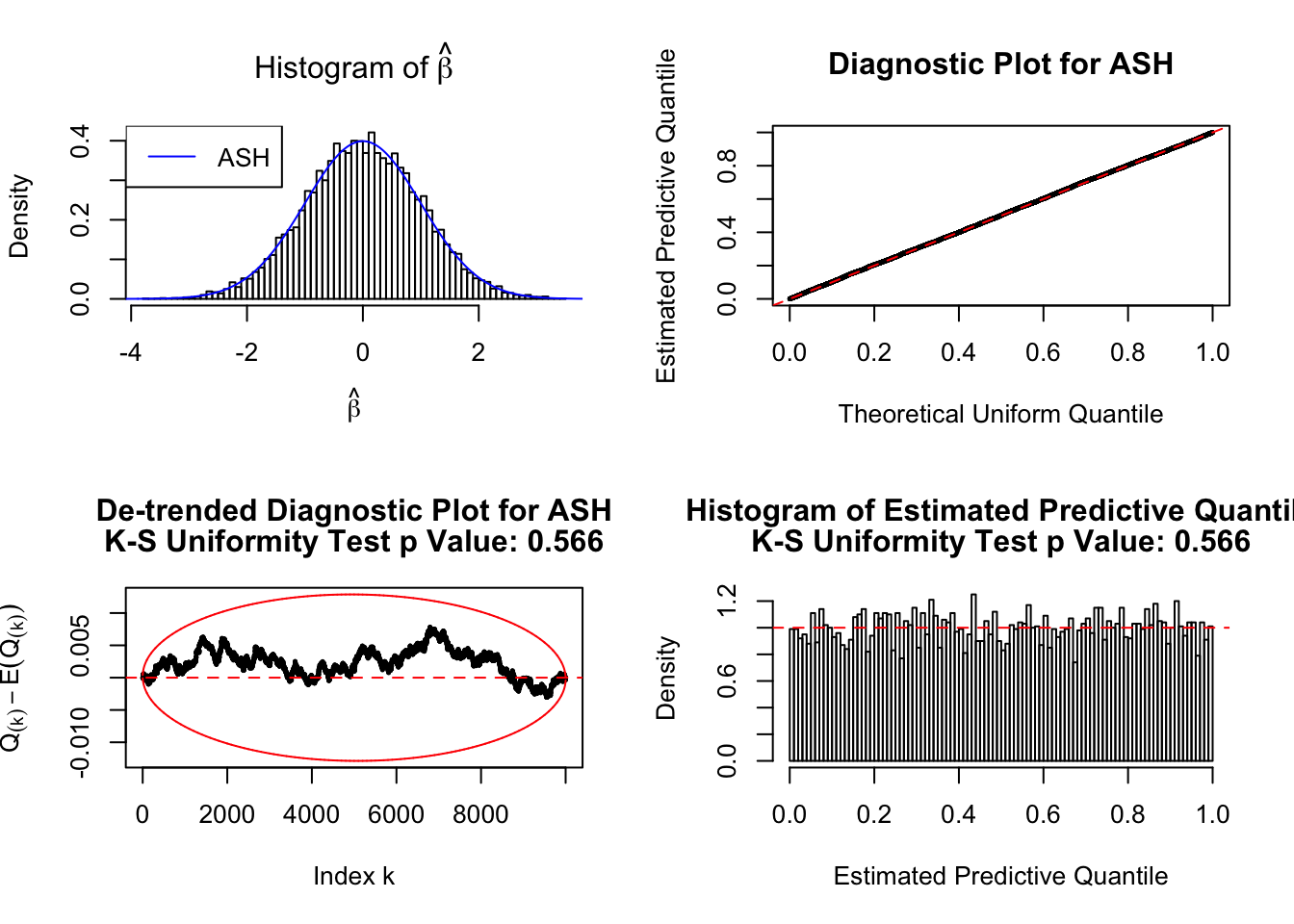

beta = sample(c(rnorm(5000, 1.5, 1), rnorm(5000, -1.5, 1)))
betahat = beta + rnorm(10000)
fit = ash(betahat, 1, mixcompdist = "normal", method = "fdr")
plot_diagnostic(fit, breaks = 100)

Press [enter] to see next plot

Press [enter] to see next plot

Press [enter] to see next plot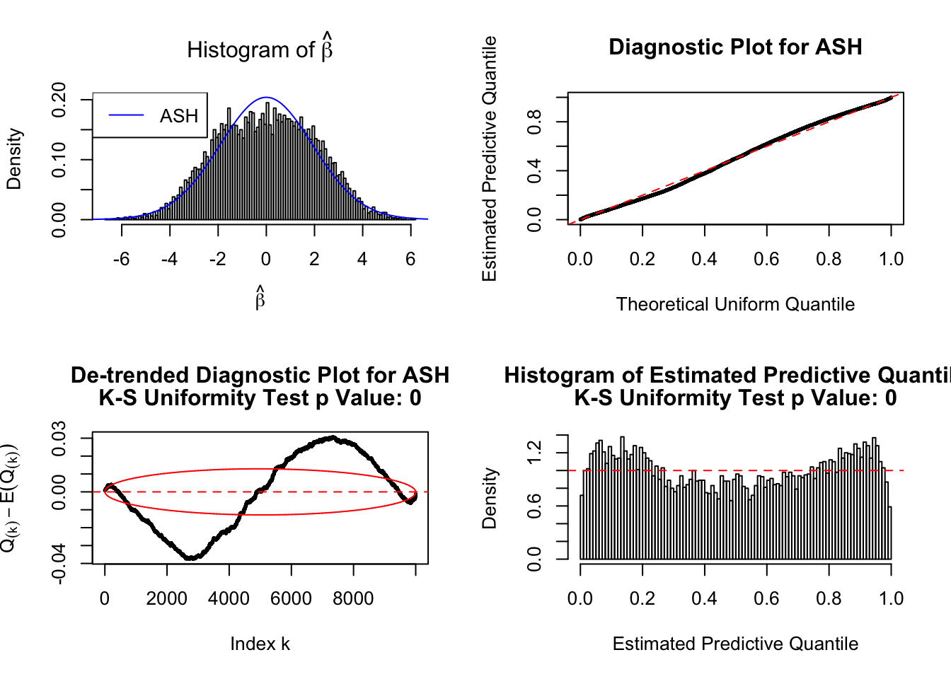

The peculiarities of the correlated null

z = readRDS("../output/z_null_liver_777_select.RDS")
z = z$typical[[5]]

hist(z, breaks = 100, prob = TRUE, xlab = "Correlated N(0, 1) Z Scores", ylim = c(0, dnorm(0)), main = "Histogram of Correlated Z Scores")
lines(seq(-6, 6, 0.01), dnorm(seq(-6, 6, 0.01)), col = "red")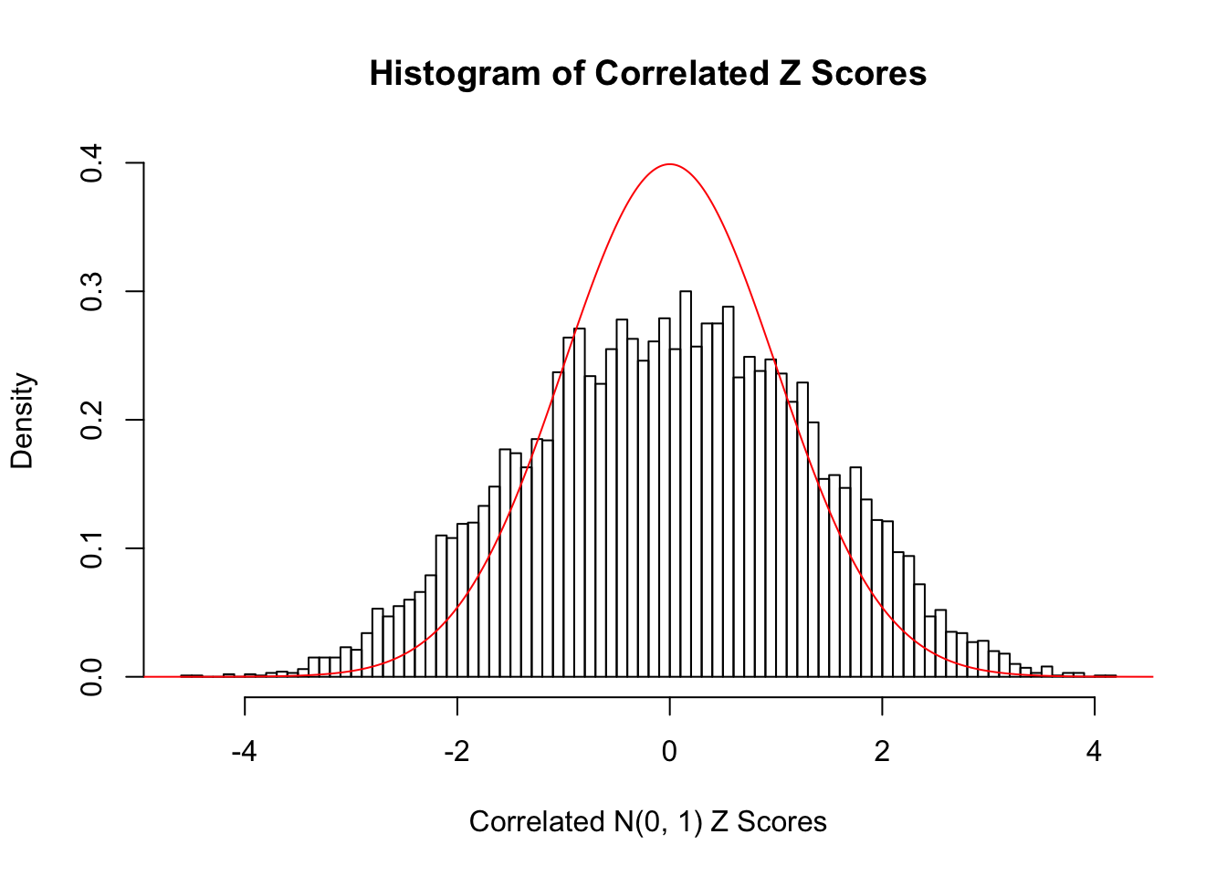

hist(z, breaks = 100, prob = TRUE, xlab = "Correlated N(0, 1) Z Scores", ylim = c(0, 0.1), main = "Histogram of Correlated Z Scores: Left Tail", xlim = c(-5, -2.5))
lines(seq(-6, 6, 0.01), dnorm(seq(-6, 6, 0.01)), col = "red")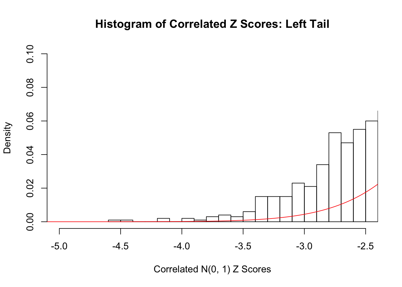

pval = (1 - pnorm(abs(z))) * 2
q = qvalue(pval)
hist(pval, breaks = 100, main = "Histogram of Correlated Z Scores' p-values", xlab = "p-values", prob = TRUE)
abline(h = q$pi0, col = "red", lty = 2)
legend("topright", lty = 2, col = "red", expression(paste(hat(pi)[0], " by qvalue")))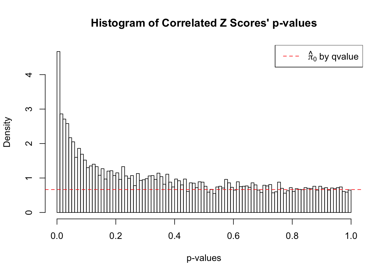

Diagnostic plots for ASH applied to the correlated null.

library(ashr)
fit = ashr::ash(z, 1, mixcompdist = "normal", method = "fdr")
par(mfrow = c(2, 2))
plot_diagnostic(fit, breaks = 100)

Press [enter] to see next plot

Press [enter] to see next plot

Press [enter] to see next plot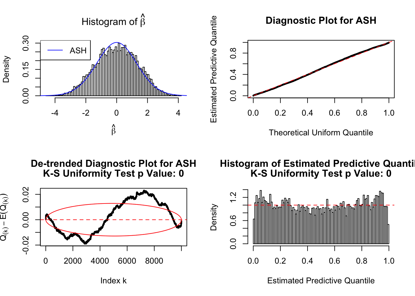

Session information

sessionInfo()

R version 3.4.3 (2017-11-30)
Platform: x86_64-apple-darwin15.6.0 (64-bit)
Running under: macOS High Sierra 10.13.2

Matrix products: default
BLAS: /Library/Frameworks/R.framework/Versions/3.4/Resources/lib/libRblas.0.dylib
LAPACK: /Library/Frameworks/R.framework/Versions/3.4/Resources/lib/libRlapack.dylib

locale:
[1] en_US.UTF-8/en_US.UTF-8/en_US.UTF-8/C/en_US.UTF-8/en_US.UTF-8

attached base packages:
[1] stats     graphics  grDevices utils     datasets  methods   base     

other attached packages:
[1] qvalue_2.10.0 ashr_2.2-2   

loaded via a namespace (and not attached):
 [1] Rcpp_0.12.14      compiler_3.4.3    git2r_0.20.0     
 [4] plyr_1.8.4        iterators_1.0.9   tools_3.4.3      
 [7] digest_0.6.13     evaluate_0.10.1   tibble_1.3.4     
[10] gtable_0.2.0      lattice_0.20-35   rlang_0.1.4      
[13] Matrix_1.2-12     foreach_1.4.4     yaml_2.1.16      
[16] parallel_3.4.3    stringr_1.2.0     knitr_1.17       
[19] REBayes_1.2       rprojroot_1.3-1   grid_3.4.3       
[22] rmarkdown_1.8     ggplot2_2.2.1     reshape2_1.4.3   
[25] magrittr_1.5      backports_1.1.2   scales_0.5.0     
[28] codetools_0.2-15  htmltools_0.3.6   MASS_7.3-47      
[31] splines_3.4.3     assertthat_0.2.0  colorspace_1.3-2 
[34] stringi_1.1.6     Rmosek_8.0.69     lazyeval_0.2.1   
[37] pscl_1.5.2        doParallel_1.0.11 munsell_0.4.3    
[40] truncnorm_1.0-7   SQUAREM_2017.10-1