Empirical Null with Gaussian Derivatives: Weight Constraints
Lei Sun
2017-03-27
Last updated: 2017-12-21
Code version: 6e42447
Numerical issues
When fitting Gaussian derivatives, overfitting or heavy correlation may cause numerical instability. Most of the time, the numerical instability leads to ridiculous weights \(w_k\), making the fitted density break the nonnegativity constraint for \(x\neq z_i\)’s.
Let normalized weights \(W_k^s = W_k\sqrt{k!}\). As shown previously, under correlated null, the variance \(\text{var}(W_k^s) = \alpha_k = \bar{\rho_{ij}^k}\). Thus, under correlated null, the Gaussian derivative decomposition of the empirical distribution should have “reasonable” weights of similar decaying patterns. In other words, \(W_k^s\) with mean \(0\) and variance \(\bar{\rho_{ij}^k}\), should be in the order of \(\sqrt{\rho^K}\) with a \(\rho\in (0, 1)\).
Examples
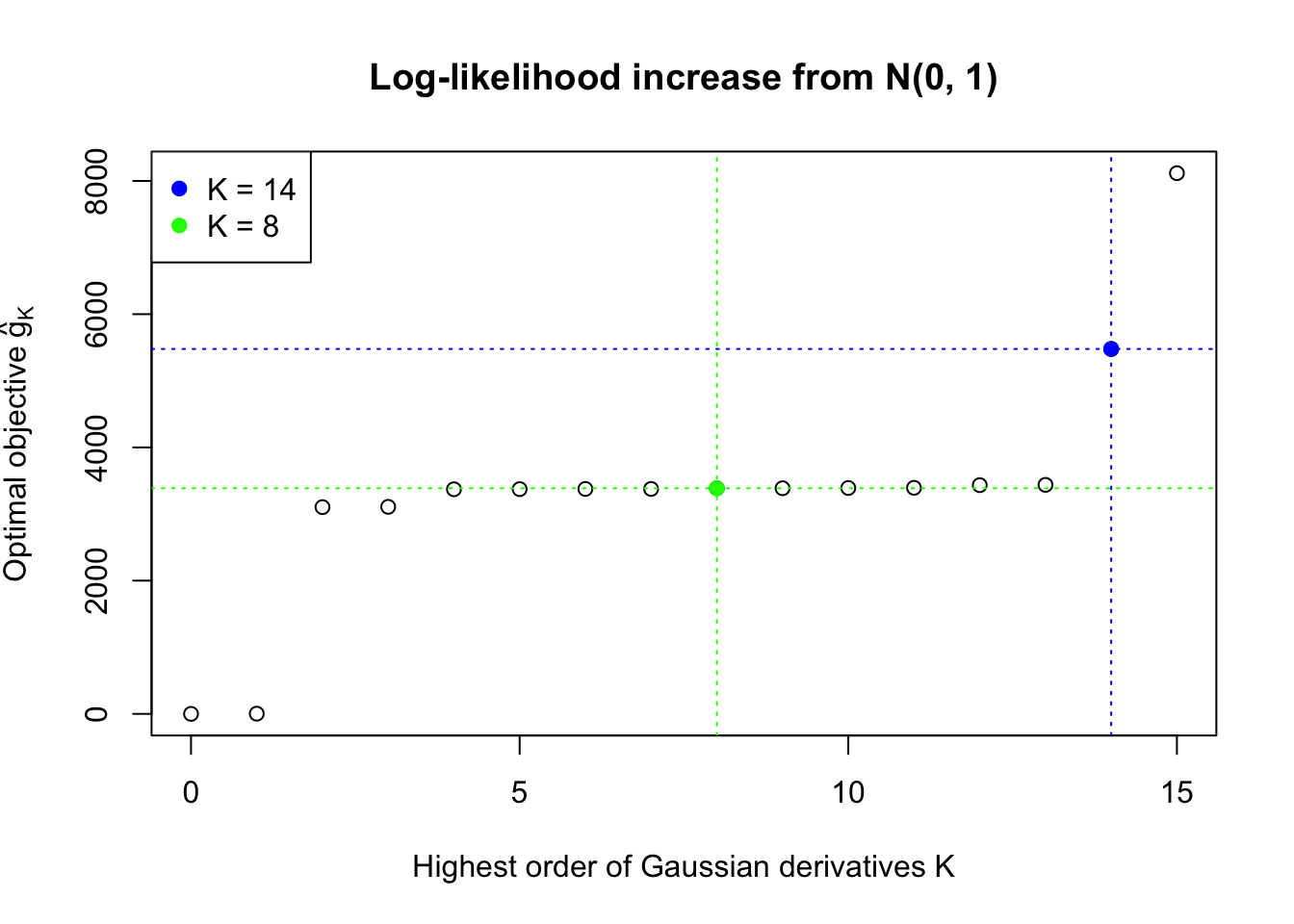
This example shows that numerical instability is reflected in the number of Gaussian derivatives fitted \(K\) being too large, as well as in the normalized fitted weights of Gaussian derivatives \(\hat w_k\sqrt{k!}\) being completely out of order \(\sqrt{\rho^K}\).
source("../code/ecdfz.R")z = read.table("../output/z_null_liver_777.txt")
p = read.table("../output/p_null_liver_777.txt")library(ashr)
DataSet = c(522, 724)
res_DataSet = list()
for (i in 1:length(DataSet)) {
zscore = as.numeric(z[DataSet[i], ])
fit.ecdfz = ecdfz.optimal(zscore)
fit.ash = ash(zscore, 1, method = "fdr")
fit.ash.pi0 = get_pi0(fit.ash)
pvalue = as.numeric(p[DataSet[i], ])
fd.bh = sum(p.adjust(pvalue, method = "BH") <= 0.05)
res_DataSet[[i]] = list(DataSet = DataSet[i], fit.ecdfz = fit.ecdfz, fit.ash = fit.ash, fit.ash.pi0 = fit.ash.pi0, fd.bh = fd.bh, zscore = zscore, pvalue = pvalue)
}library(EQL)
x.pt = seq(-5, 5, 0.01)
H.pt = sapply(1:15, EQL::hermite, x = x.pt)Data Set 724 : Number of BH's False Discoveries: 79 ; ASH's pihat0 = 0.01606004Normalized Weights for K = 8:1 : 0.0359300698579203 ; 2 : 1.08855871642562 ; 3 : 0.0779368130366434 ; 4 : 0.345861286563959 ; 5 : 0.00912636957148547 ; 6 : -0.291318682290939 ; 7 : -0.0336534605417156 ; 8 : -0.19310963474206 ;Normalized Weights for K = 14:1 : -0.676936454061805 ; 2 : -9.24968885347997 ; 3 : -8.3124954075297 ; 4 : -87.0040400264205 ; 5 : -38.5774993866502 ; 6 : -327.811119421261 ; 7 : -92.5614572826525 ; 8 : -679.045197952641 ; 9 : -123.743821656837 ; 10 : -812.599139016504 ; 11 : -88.0469137351964 ; 12 : -530.268674468285 ; 13 : -26.1051054428588 ; 14 : -146.98364434743 ;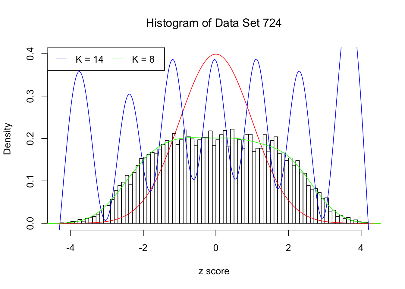
Weight constraints
Therefore, we can impose regularity in the fitted Gaussian derivatives by imposing constraints on \(w_k\). A good set of weights should have following properties.
- They should make \(\sum\limits_{k = 1}^\infty w_kh_k(x) + 1\) non-negative for \(\forall x\in\mathbb{R}\). This constraint needs to be satisfied for any distribution.
- They should decay in roughly exponential order such that \(w_k^s = w_k\sqrt{k!} \sim \sqrt{\rho^K}\). This constraint needs to be satisfied particularly for empirical correlated null.
- \(w_k\) vanishes to essentially \(0\) for sufficiently large \(k\). This constraint can be seen as coming from the last one, leading to the simplification that only first \(K\) orders of Gaussian derivatives are enough.
As Prof. Peter McCullagh pointed out during a chat, there should be a rich literature discussing the non-negativity / positivity condition for Gaussian derivative decomposition, also known as Edgeworth expansion. This could potentially be a direction to look at.
An approximation to the non-negativity constraint may come from the fact that due to orthogonality of Hermite polynomials,
\[ W_k = \frac{1}{k!}\int_{-\infty}^\infty f_0(x)h_k(x)dx \ . \] Therefore, if \(f_0\) is truly a proper density,
\[ \begin{array}{rclcl} W_1 &=& \frac{1}{1!}\int_{-\infty}^\infty f_0(x)h_1(x)dx = \int_{-\infty}^\infty x f_0(x)dx &=& E[X]_{F_0} \\ W_2 &=& \frac{1}{2!}\int_{-\infty}^\infty f_0(x)h_1(x)dx = \frac12\int_{-\infty}^\infty (x^2-1) f_0(x)dx &=& \frac12E[X^2]_{F_0} -\frac12\\ W_3 &=& \frac{1}{3!}\int_{-\infty}^\infty f_0(x)h_1(x)dx = \frac16\int_{-\infty}^\infty (x^3-3x) f_0(x)dx &=& \frac16E[X^3]_{F_0} -\frac12E[X]_{F_0}\\ W_4 &=& \frac{1}{4!}\int_{-\infty}^\infty f_0(x)h_1(x)dx = \frac1{24}\int_{-\infty}^\infty (x^4-6x^2+3) f_0(x)dx &=& \frac1{24}E[X^4]_{F_0} -\frac14E[X^2]_{F_0} + \frac18\\ &\vdots& \end{array} \] Note that \(F_0\) is not the empirical cdf \(\hat F\), even if we’ve taken into consideration that \(N\) is sufficiently large, and the correlation structure is solely determined by \(W_k\)’s and Gaussian derivatives. \(F_0\) is inherently continuous, whereas the empirical cdf \(\hat F\) is inherently non-differentiable. This implies that the mean of \(F_0\), \(E[X]_{F_0} \neq \bar X\), the mean of the empirical cdf \(\hat F\). \(W_k\)’s are still parameters of \(F_0\) that are not readily determined even given the observations (hence given the empirical cdf).
This relationship inspires the following two ways to constraint \(W_k\)’s.
Method of moments estimates
Instead of using maxmimum likelihood estimates of \(f_0\), that is, \(\max\sum\limits_{i = 1}^n\log\left(\sum\limits_{k = 1}^\infty w_kh_k(z_i) + 1\right)\), we may use method of moments estimates:
\[ \begin{array}{rcl} w_1 &=& \hat E[X]_{F_0}\\ w_2 &=& \frac12\hat E[X^2]_{F_0} -\frac12\\ w_3 &=& \frac16\hat E[X^3]_{F_0} -\frac12\hat E[X]_{F_0}\\ w_4 &=& \frac1{24}\hat E[X^4]_{F_0} -\frac14\hat E[X^2]_{F_0} + \frac18\\ &\vdots&\\ w_k &=& \cdots \end{array} \]
Constraining weights by moments
Another way is to constraint the weights by the properties of the moments to prevent them going crazy, such that
\[ W_2 = \frac12E[X^2]_{F_0} -\frac12 \Rightarrow w_2 \geq -\frac12 \ . \]
We may also combine the moment estimates and constraints like
\[ \begin{array}{rcl} w_1 &=& \hat E[X]_{F_0}\\ w_2 &\geq& -\frac12\\ &\vdots& \end{array} \] ## Quantile Constraints
It has been shown here, here, here that Benjamini-Hochberg (BH) is suprisingly robust under correlation. So Matthew has an idea to constrain the quantiles of the estimated empirical null. In his words,
I wonder if you can constrain the quantiles of the estimated null distribution using something based on BH. Eg, the estimated quantiles should be no more than \(1/\alpha\) times more extreme than expected under \(N(0,1)\) where \(\alpha\) is chosen to be the level you’d like to control FDR at under the global null.
This is not a very specific idea, but maybe gives you an idea of the kind of constraint I mean… Something to stop that estimated null having too extreme tails.
The good thing is this idea of constraining quantiles is easy to implement.
\[ \begin{array}{rcl} F_0(x) &=& \displaystyle\Phi(x) + \sum\limits_{k = 1}^\infty W_k(-1)^k \varphi^{(k - 1)}(x)\\ &=& \displaystyle\Phi(x) - \sum\limits_{k = 1}^\infty W_kh_{k-1}(x)\varphi(x) \end{array} \] So the constraints that \(F_0(x) \leq g(\alpha)\) for certain \(x, g, \alpha\) are essentially linear constraints on \(W_k\). Thus the convexity of the problem is preserved.
Implementation
Right now using the current implementation the results are disappointing. Using the constraint on \(w_2\) usually makes the optimization unstable. Using moment estimates on \(w_1\) and \(w_2\) performs better, but only sporadically.
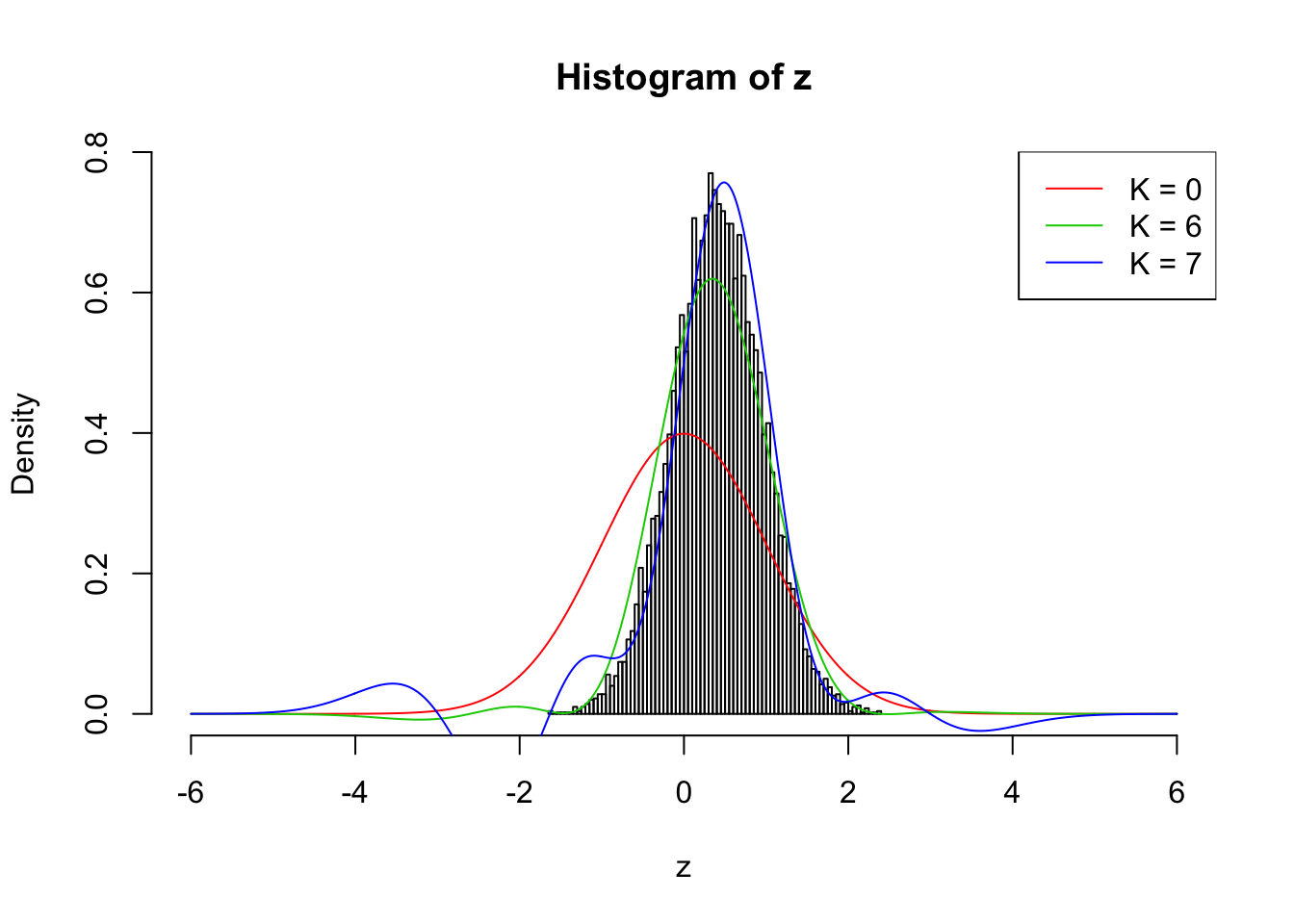
Here we are re-running the optimization on the previous \(\rho_{ij} \equiv 0.7\) example with \(\hat w_1\) and \(\hat w_2\) estimated by the method of moments. Without this tweak current implementation can only work up to \(K = 3\), which is obviously insufficient. Now it can go up to \(K = 6\). \(K = 7\) doesn’t look good, although making some improvement compared with \(K = 6\).
The results are not particularly encouraging. Right now we’ll leave it here.
rho = 0.7
set.seed(777)
n = 1e4
z = rnorm(1) * sqrt(rho) + rnorm(n) * sqrt(1 - rho)
w.3 = list()
for (ord in 6:7) {
  H = sapply(1 : ord, EQL::hermite, x = z)
  w <- Variable(ord - 2)
  w1 = mean(z)
  w2 = mean(z^2) / 2 - .5
  H2w = H[, 1:2] %*% c(w1, w2)
  objective <- Maximize(CVXR::sum_entries(CVXR::log1p(H[, 3:ord] %*% w + H2w)))
  prob <- Problem(objective)
  capture.output(result <- solve(prob), file = "/dev/null")
  w.3[[ord - 5]] = c(w1, w2, result$primal_values[[1]])
}
Conclusion
Weights \(w_k\) are of central importance in the algorithm. They contain the information regarding whether the composition of Gaussian derivatives is a proper density function, and if it is, whether it’s a correlated null. We need to find an ingenious way to impose appropriate constraints on \(w_k\).
Appendix: implementation of moments constraints
Session information
sessionInfo()R version 3.4.3 (2017-11-30)
Platform: x86_64-apple-darwin15.6.0 (64-bit)
Running under: macOS High Sierra 10.13.2
Matrix products: default
BLAS: /Library/Frameworks/R.framework/Versions/3.4/Resources/lib/libRblas.0.dylib
LAPACK: /Library/Frameworks/R.framework/Versions/3.4/Resources/lib/libRlapack.dylib
locale:
[1] en_US.UTF-8/en_US.UTF-8/en_US.UTF-8/C/en_US.UTF-8/en_US.UTF-8
attached base packages:
[1] stats graphics grDevices utils datasets methods base
other attached packages:
[1] CVXR_0.94-4 EQL_1.0-0 ttutils_1.0-1
loaded via a namespace (and not attached):
[1] Rcpp_0.12.14 knitr_1.17 magrittr_1.5
[4] bit_1.1-12 lattice_0.20-35 R6_2.2.2
[7] stringr_1.2.0 tools_3.4.3 grid_3.4.3
[10] R.oo_1.21.0 git2r_0.20.0 scs_1.1-1
[13] htmltools_0.3.6 yaml_2.1.16 bit64_0.9-7
[16] rprojroot_1.3-1 digest_0.6.13 Matrix_1.2-12
[19] gmp_0.5-13.1 ECOSolveR_0.3-2 R.utils_2.6.0
[22] evaluate_0.10.1 rmarkdown_1.8 stringi_1.1.6
[25] compiler_3.4.3 Rmpfr_0.6-1 backports_1.1.2
[28] R.methodsS3_1.7.1This R Markdown site was created with workflowr